How tree detection from a CHM works

A canopy height model (CHM) is a raster whose value at every cell is the height of the vegetation top above the ground. Detecting individual trees from it — individual tree detection, or ITD — means turning that continuous height surface into a discrete list of points — one per detected treetop, carrying its location and height. The name promises individual trees, but what a CHM reliably resolves is the canopy-dominant tree at each spot; that gap is the subject of a section below.

This page is about the ideas behind that step — what the algorithms are looking for, why there are two of them, and what you are actually trading off when you tune their parameters. For the endpoints and a runnable script, see the how-to guide Generate a tree inventory from a CHM.

The input is a height surface

Everything the detector knows comes from one band. The figure below is the NAIP-derived CHM for the Blue Mountain domain near Missoula, Montana — about 0.6 m per cell, with canopy reaching ~33 m. Bare ground and roads sit near zero; tree crowns rise as rounded mounds of height.

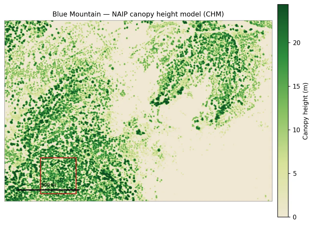
The NAIP CHM for the Blue Mountain domain. Greener cells are taller canopy; tan is near-bare ground. The red box is the 175 m window used in the close-ups below.

A CHM is a surface, not a set of stems. It does not record where one tree ends and the next begins, how many trunks produced a clump of foliage, or what species any of it is. Detection has to infer discrete trees from the shape of the surface, and every choice below follows from that one fact.

A treetop is a local maximum

The working assumption of CHM-based detection is simple: the top of a tree is a high point that is taller than everything immediately around it. Walk a window across the raster; wherever the center cell is the tallest cell in its window, call that a treetop and record a tree there.

Two parameters fall directly out of that picture:

• A height floor (min_height). Below some height, bumps in the surface are shrubs, stumps, or noise rather than trees you want in the inventory. Cells under the floor are ignored, so detection never fires on them.
• A search window. “Immediately around it” has to be made precise. The window size sets how far apart two peaks must be to count as two trees. This is the parameter with the most leverage, and it is where the two algorithms part ways.

Fixed versus variable windows

The local maxima filter (lmf) uses a fixed window — a footprint_size that is the same everywhere on the raster. It is simple, fast, and predictable: every peak is judged against a neighborhood of identical size.

The variable window filter (vwf) makes the window size a function of canopy height: tall cells are tested against a wider window, short cells against a narrower one. The motivation is biological — a 30 m tree has a much wider crown than a 5 m sapling, so the distance to its nearest distinct neighbor scales with its height. A single fixed window cannot be right for both at once: sized for the big trees it merges the small ones, sized for the small trees it splits the big ones. VWF tries to track that relationship instead of committing to one width.

Concretely the window is a straight line in height — crown_offset + crown_ratio × height — so vwf is not one window but a family of them. crown_offset is the width at zero height (the intercept); crown_ratio is how steeply the window grows with the canopy (the slope). Choosing a vwf window means choosing that slope and intercept, and the slope has real leverage: too shallow a crown_ratio keeps the window narrow even under tall trees and over-detects, while a steeper one widens the window for the overstory and merges closely-spaced peaks. The tuning guide shows how the detected count shifts as you vary it.

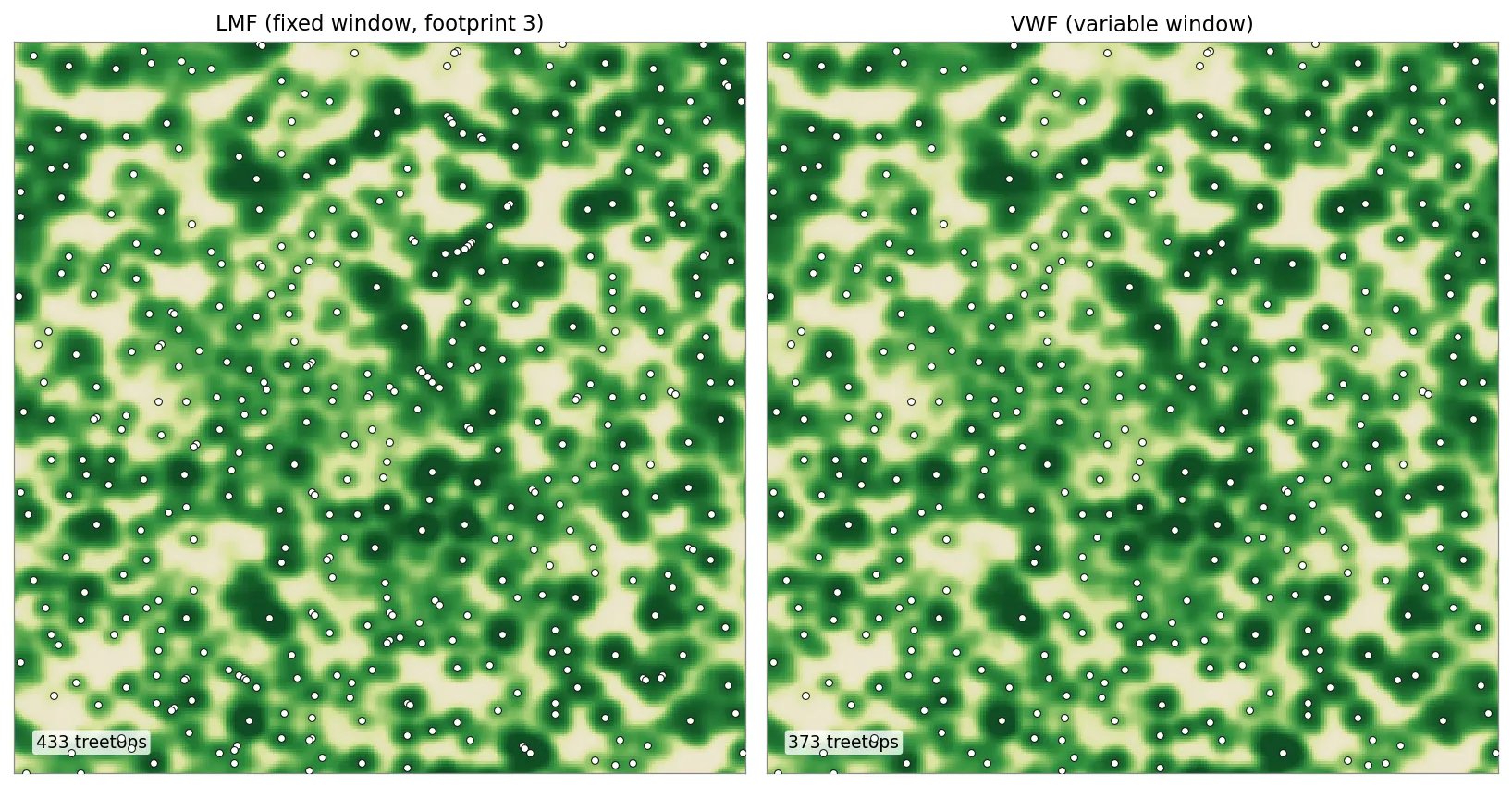
The same 175 m window detected two ways. LMF (fixed footprint) marks 433 treetops here; VWF (height-scaled window) marks 373, merging some closely-spaced peaks that the fixed window keeps separate. Across the whole domain the totals are ≈9,200 (LMF) and ≈8,500 (VWF).

Neither answer is automatically correct. Which one matches the real stand depends on how uniform the canopy is: in an even-aged plantation a fixed window is often plenty, while in a mixed-age stand with both overstory and regeneration the height-scaled window usually separates crowns more faithfully.

The over- versus under-detection trade-off

Within the fixed-window algorithm, footprint_size is the dial between two failure modes. A small window asks only that a cell beat its nearest neighbors, so it finds many peaks — including secondary bumps on a single broad crown, which show up as extra, spurious trees (over-detection). A large window forces peaks to be far apart, so neighboring trees collapse into one detection and stems go missing (under-detection).

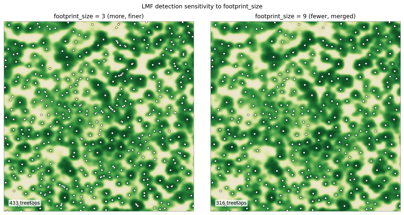
The same window at two footprint sizes. A 3-cell footprint marks 433 treetops; a 9-cell footprint marks 316, because the wider window merges adjacent peaks. Smaller footprints over-detect; larger ones under-detect.

There is no universally correct setting, because the right window is the one that matches the spacing of the trees actually on the ground — and that varies by species, age, and density. The practical way to choose is visual assessment: overlay the detected points on the CHM, as in these figures, and check whether each dot lands on a distinct crown rather than peppering one big canopy or skipping over obvious separate trees. Adjust footprint_size (or move to vwf) and min_height until the points track the crowns you can see — see Tune CHM tree detection for the export-and-overlay recipe.

Detection resolves the dominant canopy

Tuning governs the visible peaks, but a CHM has a deeper, untunable limit: it records the top of the canopy well and everything beneath it poorly. A surface seen from above is the crown exposed to the sky; a smaller tree growing under that crown leaves little or no mark on it. So a detected point is best read not as “a tree” but as the canopy-dominant tree at that spot, plus whatever it hides — the unit forestry calls a tree-approximate object.

Two consequences shape how you should read the result:

• Subordinate trees are systematically missed. Detection rate rises roughly with a tree’s height relative to its neighbors, so the understory is largely invisible. The miss rate grows with stand density — denser canopy hides more of what is below it — and in structurally complex stands it is large: studies in dense mixed-conifer forests report a median near two-thirds of stems omitted.
• A detected count is not a stem count. The missed trees are real but unseen, so the number of detections undercounts the true stems, worst exactly where the canopy is densest. Treat detections as a map of dominant crowns, not as a census of stand density.

In an open, even-aged stand one detection ≈ one tree and this barely bites; in a multi-storied or dense stand it bites hard. The detection is still the best available map of the overstory — it just is not the whole forest.

What a CHM can and cannot tell you

Because detection reads only height, a CHM-derived inventory carries only what height can support: each tree’s x, y, and height. It does not carry species or diameter at breast height — a surface seen from above never observed the trunk, and nothing in the height field distinguishes a pine from a fir of the same height.

It also reads only the top of the canopy, not its vertical profile. The height field carries no canopy base height, no bulk density, and no ladder fuels — the sub-canopy structure that carries a surface fire up into the crowns. In fire-behavior terms a CHM constrains crown-fire spread, which the overstory drives, but is silent on crown-fire initiation, which the sub-canopy drives. A CHM-derived inventory is a canopy layer, not a complete fuel column.

Note

If a downstream step needs DBH, you can estimate it from height with a height–diameter relationship (approximate, and specific to species and region), or start instead from TreeMap, which carries species composition and diameters at the cost of being a statistical sample rather than a direct observation of your canopy.

This is the core trade-off between the two inventory sources. A CHM gives you the actual canopy surface over your domain — overstory crowns where they really stand, with their heights — but only the overstory, and only its geometry. TreeMap gives you a fuller attribute set — species, DBH, crown ratio — but drawn from a model of what stands like yours typically contain. (NAIP’s CHM is itself a deep-learning estimate from imagery, not a direct measurement, so it carries its own height error — but it is anchored to your specific location.) Choose by what your simulation needs: faithful overstory geometry, or per-tree species and diameter.

Caution

For physics-based fire simulation (QUIC-Fire, FIRETEC, FDS), don’t treat the detected canopy as the whole fuelbed. A CHM resolves the overstory that drives crown-fire spread, not the sub-canopy and surface fuels that drive initiation — pair it with a statistically modeled sub-canopy and surface layer before exporting.

Where to go next

• Generate a tree inventory from a CHM — the endpoints, parameters, and a runnable two-step script.
• Generate a tree inventory from TreeMap — the species-and-diameter alternative.
• Fetch and stream the inventory data — read the detected treetops back out, one by one.