Tune CHM tree detection
You are viewing in-progress documentation for v2 (Beta). Switch to the stable version for the current production release.
Tree detection has no universally correct settings — the right footprint_size,
min_height, or VWF window depends on how your stand is spaced. The way to
choose is to look: export the CHM and the detected treetops, overlay them,
and check whether each point lands on a distinct crown. This guide runs one
round of that loop; repeat it, adjusting parameters, until the points track the
crowns you can see.
For what over- and under-detection look like — and which knob fixes each — see How tree detection from a CHM works. For the full request schema and every field default, see the live API reference.
Prerequisites
Section titled “Prerequisites”-
An API key: my-api-key.
-
A domain (your-domain-id) with a completed CHM grid (your-chm-grid-id) and at least one tree inventory (your-inventory-id) to inspect. See Generate a tree inventory from a CHM.
-
A local environment with
rasterioandmatplotlib.
Step 1 — Export the CHM and the treetops
Section titled “Step 1 — Export the CHM and the treetops”Export the CHM grid as a GeoTIFF and the inventory as GeoJSON. Both are
asynchronous: the create call returns an export in status: "pending".
curl -X 'POST' \ 'https://api-v2-prod-nyvjyh5ywa-uw.a.run.app/domains/your-domain-id/grids/your-chm-grid-id/exports/geotiff' \ -H 'accept: application/json' \ -H 'api-key: my-api-key' \ -H 'Content-Type: application/json' \ -d '{ "name": "Blue Mountain NAIP CHM", "bands": ["chm"]}'curl -X 'POST' \ 'https://api-v2-prod-nyvjyh5ywa-uw.a.run.app/domains/your-domain-id/inventories/your-inventory-id/exports/geojson' \ -H 'accept: application/json' \ -H 'api-key: my-api-key' \ -H 'Content-Type: application/json' \ -d '{ "name": "Treetops"}'Each returns an export id: your-export-id. Poll /exports/{export_id}
until status is completed, then read its signed_url.
curl -X 'GET' \ 'https://api-v2-prod-nyvjyh5ywa-uw.a.run.app/exports/your-export-id' \ -H 'accept: application/json' \ -H 'api-key: my-api-key'{ "id": "your-export-id", "domain_id": "your-domain-id", "name": "Blue Mountain NAIP CHM", "description": "", "status": "completed", "progress": { "percent": 100, "message": "Complete" }, "created_on": "2026-06-05T14:40:33.809172Z", "modified_on": "2026-06-05T14:40:36.193701Z", "source": { "bands": ["chm"], "name": "geotiff", "grid_id": "your-chm-grid-id" }, "signed_url": "https://storage.googleapis.com/silvx-fastfuels-exports-v2/your-export-id/Blue_Mountain_NAIP_CHM.tif?X-Goog-Algorithm=GOOG4-RSA-SHA256&X-Goog-Expires=604800&X-Goog-SignedHeaders=host&X-Goog-Signature=...", "expires_on": "2026-06-12T14:40:33.809172Z", "error": null, "tags": []}{ "id": "your-export-id", "domain_id": "your-domain-id", "name": "Treetops", "description": "", "status": "completed", "progress": { "percent": 100, "message": "Complete" }, "created_on": "2026-06-05T14:40:39.524329Z", "modified_on": "2026-06-05T14:40:42.579151Z", "source": { "columns": null, "crs": "EPSG:32611", "name": "geojson", "inventory_id": "your-inventory-id" }, "signed_url": "https://storage.googleapis.com/silvx-fastfuels-exports-v2/your-export-id/Treetops.geojson?X-Goog-Algorithm=GOOG4-RSA-SHA256&X-Goog-Expires=604800&X-Goog-SignedHeaders=host&X-Goog-Signature=...", "expires_on": "2026-06-12T14:40:39.524329Z", "error": null, "tags": []}The signed_url is a direct download — no API key needed, valid for seven days.
Save the two files side by side:
# paste each signed_url from the completed responses abovecurl -o chm.tif "<CHM_SIGNED_URL>"curl -o treetops.geojson "<TREETOPS_SIGNED_URL>"Step 2 — Overlay and inspect
Section titled “Step 2 — Overlay and inspect”With chm.tif and treetops.geojson in hand (both in the domain CRS), plot the
treetops over a close-up of the CHM:
"""Overlay detected treetops on the CHM to judge detection quality.
Reads the two files you downloaded from the export signed URLs:  chm.tif          — the exported CHM grid (geotiff)  treetops.geojson — the exported tree inventory (geojson, same CRS)
Writes overlay.png: detected treetops as dots over a close-up of the CHM.Run it for each candidate inventory and compare the overlays."""import json
import matplotlib.pyplot as pltimport numpy as npimport rasterio
WINDOW_M = 175.0  # side length of the close-up window, in CHM map units (m)
with rasterio.open("chm.tif") as src:    chm = src.read(1, masked=True)    b = src.bounds    extent = (b.left, b.right, b.bottom, b.top)
# A close-up window — small enough that individual treetops are legible.x0, y0 = b.left + 175.0, b.bottom + 40.0x1, y1 = x0 + WINDOW_M, y0 + WINDOW_M
pts = np.array([    f["geometry"]["coordinates"][:2]    for f in json.load(open("treetops.geojson"))["features"]])inside = (pts[:, 0] >= x0) & (pts[:, 0] <= x1) & (pts[:, 1] >= y0) & (pts[:, 1] <= y1)
fig, ax = plt.subplots(figsize=(7, 7))ax.imshow(chm, extent=extent, origin="upper", cmap="Greens",          vmax=np.percentile(chm.compressed(), 99))ax.scatter(pts[inside, 0], pts[inside, 1], s=14,           facecolor="white", edgecolor="black", linewidth=0.5)ax.set_xlim(x0, x1)ax.set_ylim(y0, y1)ax.set_xticks([])ax.set_yticks([])ax.set_title(f"{int(inside.sum())} treetops in a {WINDOW_M:.0f} m window")fig.savefig("overlay.png", dpi=150, bbox_inches="tight")print(f"{int(inside.sum())} treetops in view -> overlay.png")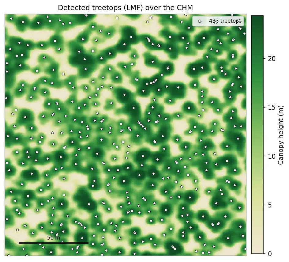
A real, untuned result — not an ideal one. The dots track local height peaks, but in this dense canopy the crowns merge into a near-continuous surface, so some connected crowns carry several dots and the boundaries between trees are ambiguous. Weighing trade-offs like these is the point of inspecting the overlay.
Step 3 — Read it and adjust
Section titled “Step 3 — Read it and adjust”Compare the dots to the canopy and re-create the inventory with new parameters:
- Several dots on one crown (over-detection) → enlarge
footprint_size, or switch tovwf. - Obvious trees with no dot (under-detection) → shrink
footprint_size. - Dots on low shrubs or understory → raise
min_height. - Dots on rooftops or powerlines → NAIP-CHM includes structures; mask them (e.g. with building footprints) or restrict the domain to vegetated land.
Each knob moves the count in a predictable direction. On the Blue Mountain
domain (≈1 km², NAIP CHM, min_height 2 m), holding everything else fixed, the
whole-domain treetop count responds like this:
lmf footprint_size (px) | treetops |
|---|---|
| 3 | 9,227 |
| 5 | 7,836 |
| 7 | 7,345 |
| 9 | 6,898 |
A wider footprint forces peaks farther apart, so neighboring crowns merge and
the count falls. vwf instead grows the window with canopy height; its
crown_ratio sets how fast (window = crown_offset + crown_ratio × height):
vwf crown_ratio (at crown_offset 1.0) | treetops |
|---|---|
| 0.05 | 37,381 |
| 0.10 | 8,506 |
| 0.15 | 8,099 |
| 0.20 | 7,818 |
A small crown_ratio keeps the window narrow even under tall canopy, so it
over-detects sharply — the 0.05 row finds roughly four times as many treetops
as 0.10. Raising it widens the window for tall trees and brings the count down.
These are one stand’s numbers, not targets: the right setting is the one whose
dots track the crowns in your overlay.
Then overlay again. Side-by-side examples of each effect — fixed vs. variable window, and the footprint-size trade-off — are in How tree detection from a CHM works.
These knobs balance detection of the visible canopy. Trees occluded beneath the dominant crowns can’t be recovered by tuning — see Detection resolves the dominant canopy for why a detected count undercounts the true stems.