Generate a tree inventory from a CHM
You are viewing in-progress documentation for v2 (Beta). Switch to the stable version for the current production release.
When you have a canopy height model (CHM) — a raster of vegetation height — you can detect individual trees from it directly, rather than sampling them statistically from TreeMap. FastFuels does this in two steps:
- Build a CHM grid — worked through below with NAIP aerial imagery
(
canopy/naip), a ~0.6 m canopy height model covering the conterminous US. It is one of several sources; see Choosing a source. - Isolate stems — run a tree-detection algorithm over the CHM to place
one tree at each detected treetop (
tree/chm).
For the ideas behind step 2 — why a treetop is a local maximum, and how the two algorithms differ — see How tree detection from a CHM works.
Prerequisites
Section titled “Prerequisites”-
An API key: my-api-key.
-
A domain: your-domain-id. See Create a domain.
Choosing a source
Section titled “Choosing a source”Four canopy constructors emit a chm band, and a fifth route lets you bring your
own raster. Any of them can feed Step 2:
| Source | Endpoint | Cell size | What it is |
|---|---|---|---|
| NAIP | grids/canopy/naip | ~0.6 m | A deep-learning canopy height model derived from aerial imagery. CONUS only. Used in Step 1 below. |
| Meta | grids/canopy/meta | ~1 m | A deep-learning canopy height model with global coverage. |
| Airborne lidar | grids/canopy/point_cloud | 1 m or coarser | Rasterized from a point cloud you fetched from 3DEP or uploaded. A direct measurement rather than a model. |
| LANDFIRE | grids/canopy/landfire | 30 m | A national canopy layer carrying chm alongside cbd, cbh, and cc. Too coarse for individual-tree detection — a 30 m cell is wider than a crown. |
| Your own raster | grids/upload/geotiff | whatever you supply | Any CHM the API does not produce itself. |
Two things decide the choice more often than quality does:
- Coverage. The lidar route needs a point cloud, and 3DEP does not cover everywhere. Of six 1 km² boxes we tried around Missoula, Montana, three had 3DEP lidar and three had none — including the Blue Mountain domain used throughout these guides. Check coverage before you plan around it. NAIP and Meta have no such gap.
- Cell size against crown size. Detection resolves peaks in a raster, so a cell must be well inside a crown for a crown to have a peak. That rules LANDFIRE out for this job and makes it the wrong tool here, however good it is for stand-scale canopy fuel.
Step 1 — Build the CHM grid
Section titled “Step 1 — Build the CHM grid”NAIP imagery is processed by a deep-learning model into a ~0.6 m canopy height surface, so this grid is fine-grained. It is a modeled surface (≈1 m typical height error) that also captures buildings and other tall structures — see Common pitfalls. No version or band selection is needed — the source resolves the NAIP-CHM tiles that cover your domain.
curl -X 'POST' \ 'https://api-v2-prod-nyvjyh5ywa-uw.a.run.app/domains/your-domain-id/grids/canopy/naip' \ -H 'accept: application/json' \ -H 'api-key: my-api-key' \ -H 'Content-Type: application/json' \ -d '{ "name": "NAIP CHM"}'import fastfuels_sdk.v2 as ff
ff.set_api_key("my-api-key")
domain = ff.Domain.from_id("your-domain-id")
chm = ff.grids.create_canopy_height_grid_from_naip_chm(domain, name="NAIP CHM")chm.wait()Poll to completed and record the grid id: your-chm-grid-id.
{ "id": "your-chm-grid-id", "domain_id": "your-domain-id", "name": "NAIP CHM", "description": "", "status": "completed", "progress": { "percent": 100, "message": "Complete" }, "created_on": "2026-10-13T02:04:36.391401Z", "modified_on": "2026-10-13T02:04:47.490667Z", "checksum": "679ac763106440f998d563f5afe8f97c", "source": { "tile_metadata": { "tile_count": 1, "native_crs": "EPSG:32611", "tiles": [ "https://rangeland.ntsg.umt.edu/data/naip-chm/2023/11/m_4611416_nw_11_060_20231019_20240103_chm.tif" ], "acquisition_dates": null, "tile_source": null }, "alignment": { "method": null, "target": "domain", "resolution": null }, "name": "canopy", "description": "NAIP high-resolution canopy height model at ~0.6m resolution (CONUS)", "extent_buffer_cells": 0, "product": "naip" }, "modifications": [], "bands": [ { "key": "chm", "name": "Canopy Height", "description": "Height above ground of the canopy top.", "type": "continuous", "unit": "m", "index": 0, "nodata": null, "summary": { "type": "continuous", "count": 3216975, "nodata_count": 0, "min": 0.0, "max": 32.689998626708984, "mean": 5.950183918105713, "std": 7.25633903389633 } } ], "georeference": { "crs": "EPSG:32611", "transform": [ 0.5997260672151095, 0.0, 720226.0, 0.0, -0.5997260672150779, 5190646.595949142 ], "shape": [1475, 2181] }, "error": null, "chunks": { "shape": [512, 512], "count": 15, "count_by_axis": { "x": 5, "y": 3 } }, "tags": []}The grid carries a single chm band (canopy height, in meters).
Step 2 — Isolate stems
Section titled “Step 2 — Isolate stems”Point source_chm_grid_id at the completed CHM grid and pick a stem-isolation
algorithm:
lmf(local maxima filter) — finds treetops as local height maxima within a fixedfootprint_sizewindow; ignores anything belowmin_height.vwf(variable window filter) — scales the search window with canopy height, which separates large and small crowns better in mixed stands. The window diameter in meters iscrown_offset+crown_ratio× height. The defaults arecrown_offset3.0 andcrown_ratio0.05.
Pick your algorithm below. For the full request schema and every field default, see the live API reference.
curl -X 'POST' \ 'https://api-v2-prod-nyvjyh5ywa-uw.a.run.app/domains/your-domain-id/inventories/tree/chm' \ -H 'accept: application/json' \ -H 'api-key: my-api-key' \ -H 'Content-Type: application/json' \ -d '{ "name": "Tree inventory from CHM", "source_chm_grid_id": "your-chm-grid-id", "algorithm": { "name": "lmf", "min_height": 2, "footprint_size": 3 }}'from fastfuels_sdk.v2.client_library.models import StemIsolationLmf
inventory = ff.inventories.create_tree_inventory_from_chm_grid( domain, chm, algorithm=StemIsolationLmf(min_height=2, footprint_size=3), name="Tree inventory from CHM",){ "id": "your-inventory-id", "domain_id": "your-domain-id", "type": "tree", "name": "Tree inventory from CHM", "description": "", "status": "pending", "progress": null, "created_on": "2026-10-13T02:22:06.682457", "modified_on": "2026-10-13T02:22:06.682457", "checksum": "e4c4c9adb9014ff7be94132c05891316", "source": { "name": "chm", "source_chm_grid_id": "your-chm-grid-id", "source_chm_grid_checksum": "679ac763106440f998d563f5afe8f97c", "algorithm": { "name": "lmf", "min_height": 2.0, "max_height": 120.0, "footprint_size": 3 }, "crown_segmentation": null }, "modifications": [], "treatments": [], "columns": [ { "key": "tree_id", "type": "categorical", "unit": null, "summary": null }, { "key": "x", "type": "continuous", "unit": "m", "summary": null }, { "key": "y", "type": "continuous", "unit": "m", "summary": null }, { "key": "height", "type": "continuous", "unit": "m", "summary": null } ], "forestry_metrics": null, "georeference": null, "error": null, "tags": []}curl -X 'POST' \ 'https://api-v2-prod-nyvjyh5ywa-uw.a.run.app/domains/your-domain-id/inventories/tree/chm' \ -H 'accept: application/json' \ -H 'api-key: my-api-key' \ -H 'Content-Type: application/json' \ -d '{ "name": "Tree inventory from CHM", "source_chm_grid_id": "your-chm-grid-id", "algorithm": { "name": "vwf", "min_height": 2, "crown_ratio": 0.05, "crown_offset": 3.0 }}'from fastfuels_sdk.v2.client_library.models import StemIsolationVwf
inventory = ff.inventories.create_tree_inventory_from_chm_grid( domain, chm, algorithm=StemIsolationVwf(min_height=2, crown_ratio=0.05, crown_offset=3.0), name="Tree inventory from CHM",){ "id": "your-inventory-id", "domain_id": "your-domain-id", "type": "tree", "name": "Tree inventory from CHM", "description": "", "status": "pending", "progress": null, "created_on": "2026-10-13T02:22:11.396783", "modified_on": "2026-10-13T02:22:11.396783", "checksum": "2d67193348954dcea2853b08af49d2bc", "source": { "name": "chm", "source_chm_grid_id": "your-chm-grid-id", "source_chm_grid_checksum": "679ac763106440f998d563f5afe8f97c", "algorithm": { "name": "vwf", "min_height": 2.0, "max_height": 120.0, "spatial_resolution": null, "crown_ratio": 0.05, "crown_offset": 3.0 }, "crown_segmentation": null }, "modifications": [], "treatments": [], "columns": [ { "key": "tree_id", "type": "categorical", "unit": null, "summary": null }, { "key": "x", "type": "continuous", "unit": "m", "summary": null }, { "key": "y", "type": "continuous", "unit": "m", "summary": null }, { "key": "height", "type": "continuous", "unit": "m", "summary": null } ], "forestry_metrics": null, "georeference": null, "error": null, "tags": []}Record the inventory id: your-inventory-id. Poll until completed:
curl -X 'GET' \ 'https://api-v2-prod-nyvjyh5ywa-uw.a.run.app/domains/your-domain-id/inventories/your-inventory-id' \ -H 'accept: application/json' \ -H 'api-key: my-api-key'inventory.wait(){ "id": "your-inventory-id", "domain_id": "your-domain-id", "type": "tree", "name": "Tree inventory from CHM", "description": "", "status": "completed", "progress": { "percent": 100, "message": "Complete" }, "created_on": "2026-10-13T02:22:06.682457Z", "modified_on": "2026-10-13T02:22:09.121913Z", "checksum": "e4c4c9adb9014ff7be94132c05891316", "source": { "algorithm": { "footprint_size": 3, "name": "lmf", "min_height": 2.0, "max_height": 120.0 }, "name": "chm", "source_chm_grid_checksum": "679ac763106440f998d563f5afe8f97c", "crown_segmentation": null, "source_chm_grid_id": "your-chm-grid-id" }, "modifications": [], "treatments": [], "columns": [ { "key": "tree_id", "type": "categorical", "unit": null, "summary": { "type": "categorical", "count": 8040, "null_count": 0, "unique_count": 8040 } }, { "key": "x", "type": "continuous", "unit": "m", "summary": { "type": "continuous", "count": 8040, "null_count": 0, "min": 720226.2998630336, "max": 721533.7026895626, "mean": 720773.5308036121, "std": 366.6012326050068 } }, { "key": "y", "type": "continuous", "unit": "m", "summary": { "type": "continuous", "count": 8040, "null_count": 0, "min": 5189762.299863034, "max": 5190646.296086108, "mean": 5190228.973942304, "std": 250.60501047478576 } }, { "key": "height", "type": "continuous", "unit": "m", "summary": { "type": "continuous", "count": 8040, "null_count": 0, "min": 2.009999990463257, "max": 32.689998626708984, "mean": 14.77024502920274, "std": 6.678434829870902 } } ], "forestry_metrics": null, "georeference": { "crs": "EPSG:32611", "bounds": [720226.0, 5189762.0, 721534.0, 5190646.0] }, "error": null, "tags": []}On the Blue Mountain domain, lmf with a 3-pixel footprint and a 2 m minimum
detects 8,040 treetops; vwf with the default window detects 7,369.
These are overstory detections, not a full stem count — trees beneath the
dominant canopy aren’t seen (why).
The inventory’s data columns are tree_id, x, y, and height — an id,
position and treetop height, the observables a CHM provides.
Both counts are specific to this CHM at this cell size. footprint_size is
measured in pixels, so a 3-pixel footprint is 1.8 m on this 0.6 m NAIP grid and
would be 3 m on a 1 m lidar grid — and the surfaces differ in more than their
lattice. The source changes the answer shows
how far apart the same request lands on two sources.
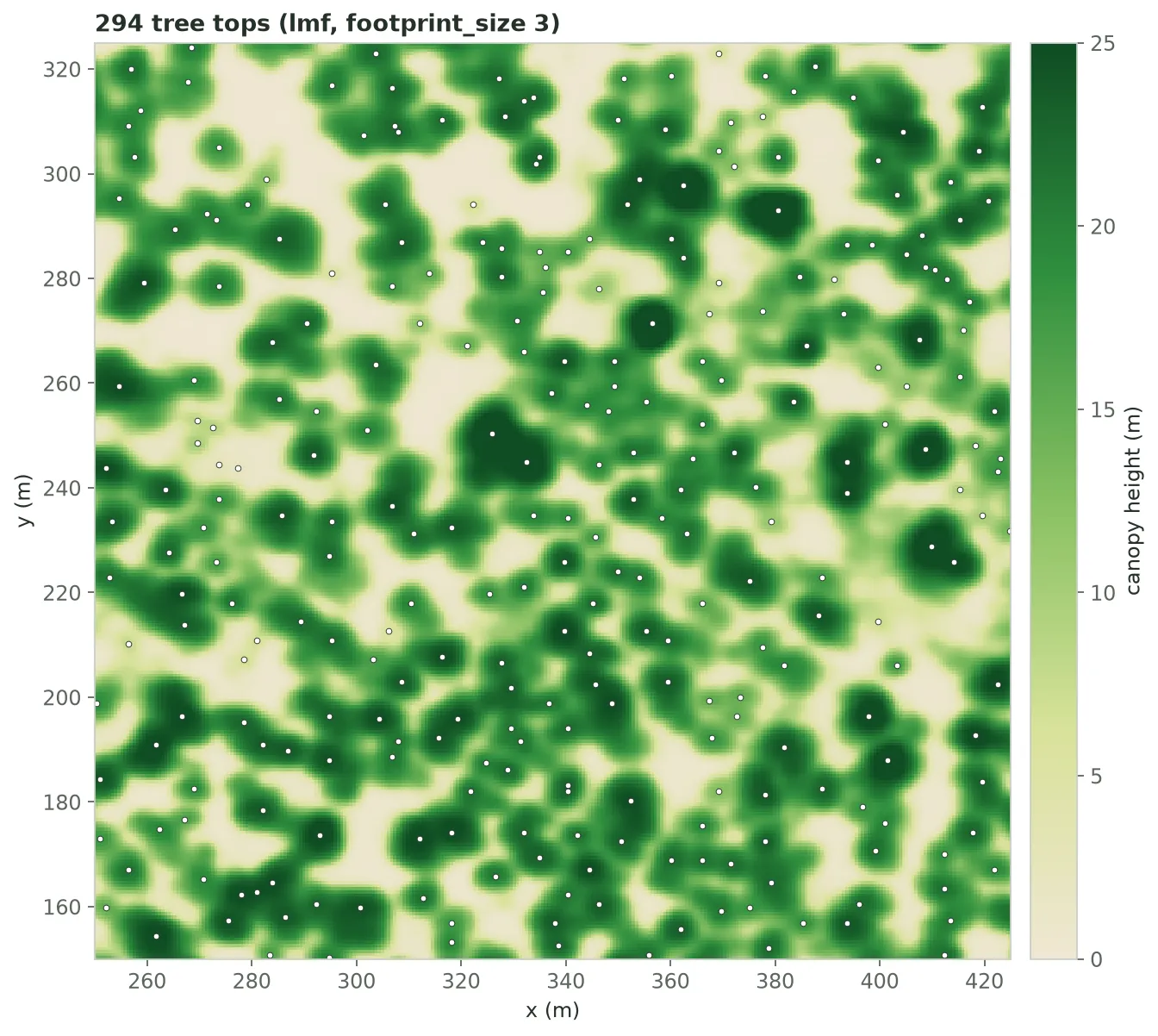
Detected treetops (LMF, footprint_size 3) over the NAIP CHM, a 175 m
window of the Blue Mountain domain. Each dot is one row of the inventory,
placed at a local height maximum. Brighter cells are taller canopy.
Measure each tree’s crown radius
Section titled “Measure each tree’s crown radius”Add crown_segmentation to the request to measure each tree’s crown on the
CHM. Each crown grows outward from its treetop over the CHM cells, within the
detection height range, until it reaches the crown’s edge. Each cell belongs to
at most one tree. The inventory gets a crown_radius column (m): the radius of
a circle with the crown’s area. Each radius is at least that of one CHM cell
and at most max_crown_radius (10 m by default).
The CHM grid must be at 2 m resolution or finer, or the request returns 422.
{} uses the defaults; the
API reference lists every
field.
curl -X 'POST' \ 'https://api-v2-prod-nyvjyh5ywa-uw.a.run.app/domains/your-domain-id/inventories/tree/chm' \ -H 'accept: application/json' \ -H 'api-key: my-api-key' \ -H 'Content-Type: application/json' \ -d '{ "name": "Tree inventory from CHM, with crown radius", "source_chm_grid_id": "your-chm-grid-id", "algorithm": { "name": "lmf", "min_height": 2, "footprint_size": 3 }, "crown_segmentation": {}}'from fastfuels_sdk.v2.client_library.models import StemIsolationLmf
inventory = ff.inventories.create_tree_inventory_from_chm_grid( domain, chm, algorithm=StemIsolationLmf(min_height=2, footprint_size=3), crown_segmentation={}, name="Tree inventory from CHM, with crown radius",)inventory.wait(){ "id": "your-inventory-id", "domain_id": "your-domain-id", "type": "tree", "name": "Tree inventory from CHM, with crown radius", "description": "", "status": "completed", "progress": { "percent": 100, "message": "Complete" }, "created_on": "2026-10-13T02:22:16.265404Z", "modified_on": "2026-10-13T02:22:19.802177Z", "checksum": "89f40d89366741fd825d6fe040d56d68", "source": { "algorithm": { "footprint_size": 3, "name": "lmf", "min_height": 2.0, "max_height": 120.0 }, "name": "chm", "source_chm_grid_checksum": "679ac763106440f998d563f5afe8f97c", "crown_segmentation": { "method": "dalponte2016", "min_relative_height": 0.45, "max_crown_radius": 10.0, "radius_estimator": "area_equivalent", "min_relative_crown_height": 0.55 }, "source_chm_grid_id": "your-chm-grid-id" }, "modifications": [], "treatments": [], "columns": [ { "key": "tree_id", "type": "categorical", "unit": null, "summary": { "type": "categorical", "count": 8040, "null_count": 0, "unique_count": 8040 } }, { "key": "x", "type": "continuous", "unit": "m", "summary": { "type": "continuous", "count": 8040, "null_count": 0, "min": 720226.2998630336, "max": 721533.7026895626, "mean": 720773.5308036121, "std": 366.60123260500757 } }, { "key": "y", "type": "continuous", "unit": "m", "summary": { "type": "continuous", "count": 8040, "null_count": 0, "min": 5189762.299863034, "max": 5190646.296086108, "mean": 5190228.973942304, "std": 250.60501047481839 } }, { "key": "height", "type": "continuous", "unit": "m", "summary": { "type": "continuous", "count": 8040, "null_count": 0, "min": 2.009999990463257, "max": 32.689998626708984, "mean": 14.77024502920274, "std": 6.678434829870902 } }, { "key": "crown_radius", "type": "continuous", "unit": "m", "summary": { "type": "continuous", "count": 8040, "null_count": 0, "min": 0.3383592001048174, "max": 8.68601743762824, "mean": 4.095841335962233, "std": 1.1426696436618209 } } ], "forestry_metrics": null, "georeference": { "crs": "EPSG:32611", "bounds": [720226.0, 5189762.0, 721534.0, 5190646.0] }, "error": null, "tags": []}The same 8,040 trees come back, now with a crown_radius column.
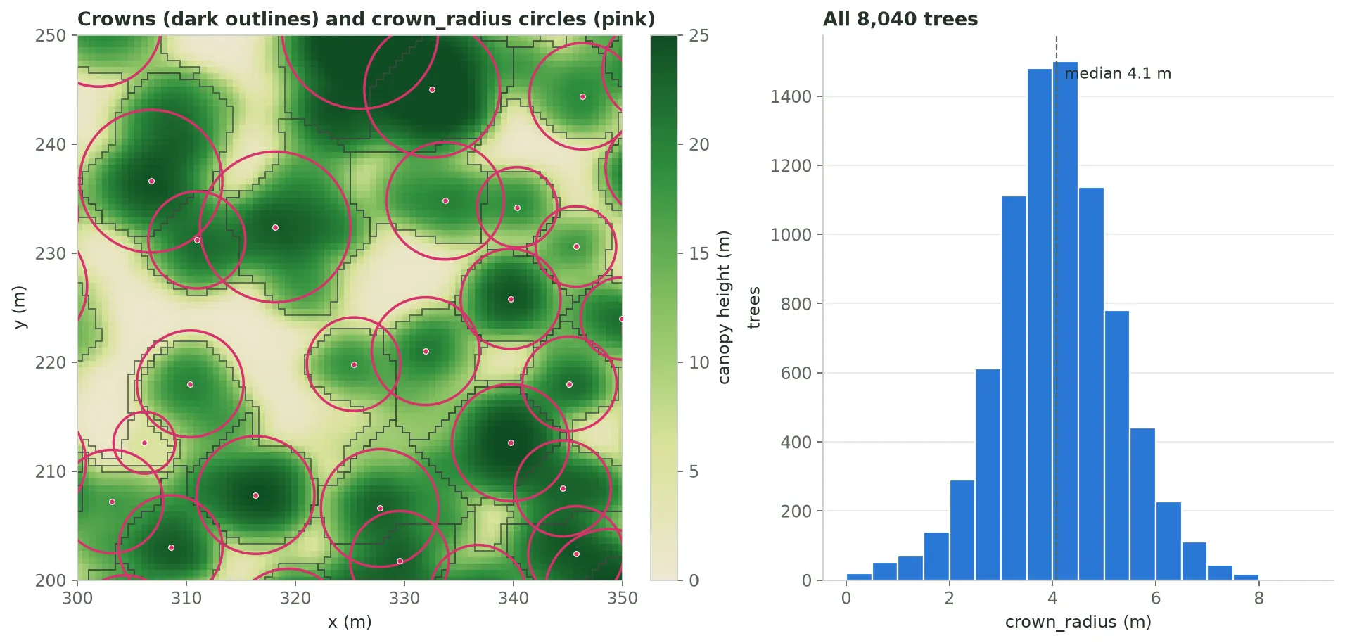
Left: each tree’s measured crown (white outline) and a circle with its
crown_radius (pink). The circle has the crown’s area, not its shape.
Right: crown_radius across the Blue Mountain domain.
To use the radius, complete the inventory with
GDAM,
which keeps the crown_radius column, then
voxelize it with measured crown radii.
To keep each crown’s full outline instead of one radius,
create a crown Feature
from the inventory and the CHM grid. For how the two compare, see
Where crown geometry comes from.
The source changes the answer
Section titled “The source changes the answer”Those counts belong to a NAIP CHM at 0.6 m. Run the same request against a CHM built from lidar and you get a different inventory of the same forest.
Here is that comparison on a domain that has both: the 53 ha Blackfoot River
domain from From lidar to a tree inventory,
east of Missoula, Montana. It has a NAIP CHM and a 1 m CHM built from 3DEP
lidar. Both are detected with identical parameters (lmf, footprint_size
3, min_height 2 m):
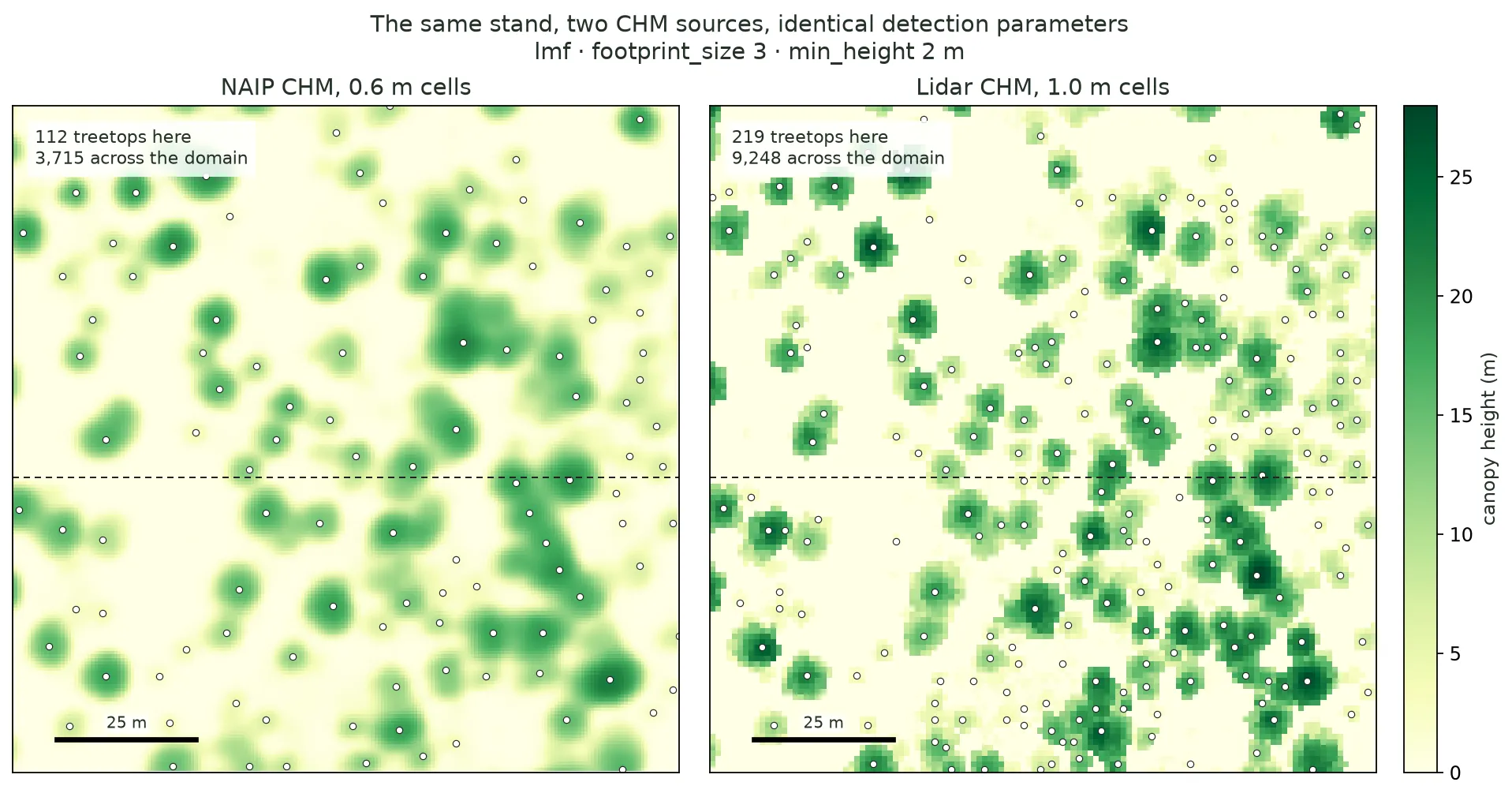
The same 120 m stand. NAIP detects 3,715 treetops across the domain; the lidar CHM detects 9,248, 2.5× more, from the same request body.
The reason is visible in the panels. NAIP is a modeled surface: a network predicts a height for every pixel, and it predicts smoothly, so a crown is a round mound with one summit. The lidar CHM is a measurement: each cell holds the tallest return that happened to land in it, so a crown is a rough cluster of peaks and troughs. A local-maxima filter counts summits, and one of these surfaces has far more of them.
That roughness is measurable. Over canopy cells, in a matched 3 m ground window, the mean local height standard deviation is 1.8 m for NAIP and 2.9 m for the lidar CHM.
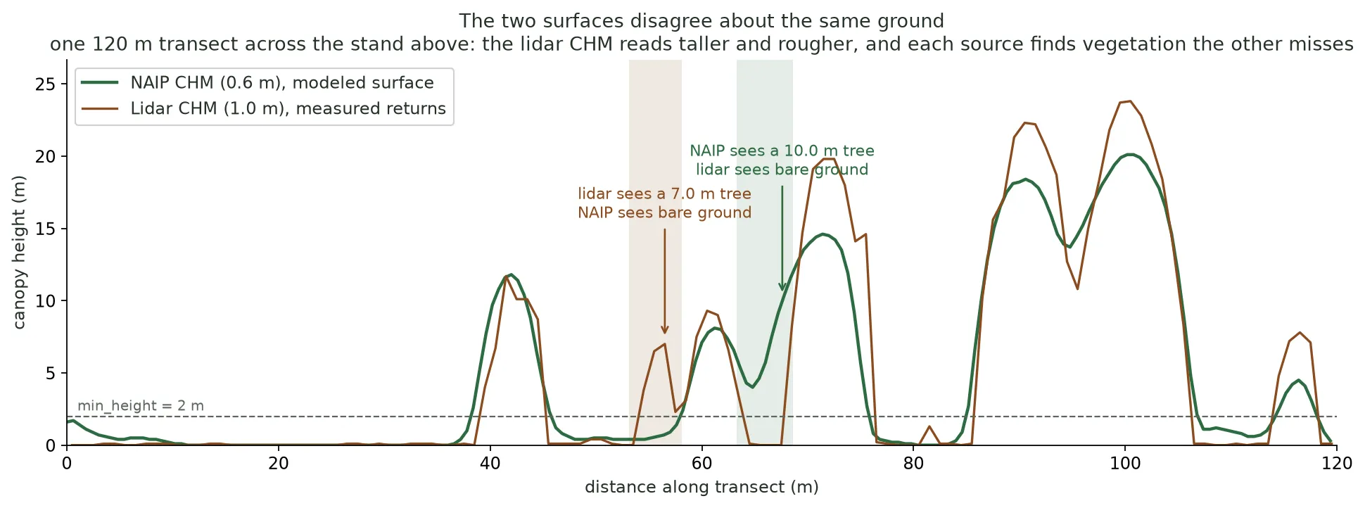
The transect marked in the stand above. The lidar CHM reads taller on the same crowns, 23.8 m against 20.1 m on the tallest, and the two sources disagree outright twice in 120 m, in both directions.
It is not just the cell size
Section titled “It is not just the cell size”footprint_size is measured in pixels, so the same number is a different
distance on the ground: 3 px is 1.8 m on a 0.6 m NAIP grid and 3.0 m on a 1 m
lidar grid. That matters, and it is worth correcting for — but correcting for it
does not close the gap.
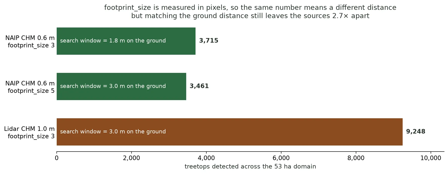
Widening NAIP’s footprint to 5 px matches the lidar run’s 3 m search window and drops NAIP to 3,461, still 2.7× fewer than the lidar CHM. The difference is in the surfaces, not only in the lattice.
Nor is the gap confined to short vegetation that one source resolves and the other smooths away. Every height band gains:
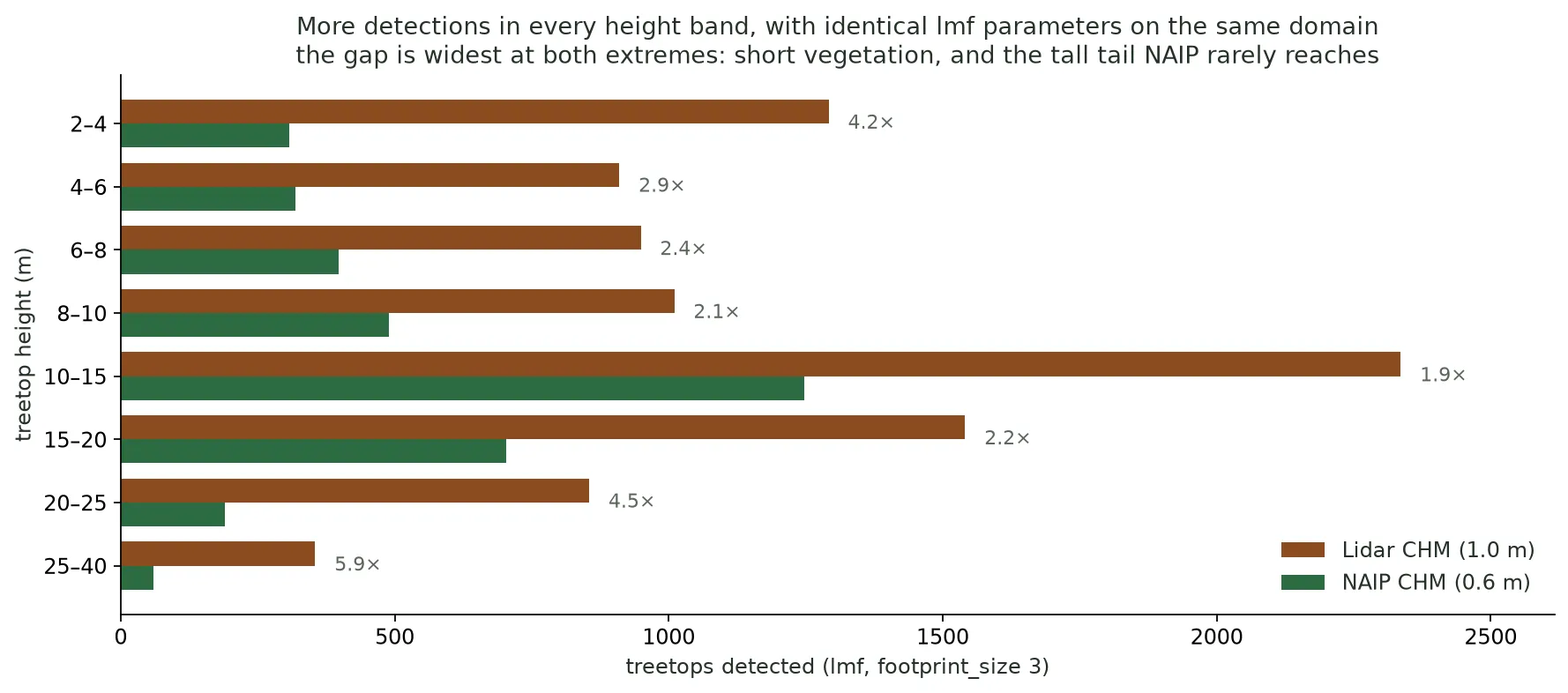
Detected treetops by height. The gap is widest at both ends: 4.2× among 2–4 m treetops, and 5.9× above 25 m, where NAIP’s modeled surface rarely reaches. Its 99th percentile canopy height is 24.3 m, against 28.3 m for the lidar CHM.
What to do with this. Neither count is the true stem count, and neither is “the correct one”. The lidar CHM’s 175 detections per hectare include detections on low vegetation and on a power line, and NAIP’s smoothing hides real stems. Treat the source and the parameters as one choice, not two:
-
Re-tune whenever you change source. Parameters carried over from another CHM are not a starting point, they are a different question. Inspect the overlay and adjust until the dots track the crowns in this raster.
-
Convert
footprint_sizeto metres before comparing settings — multiply by the grid’s cell size. Two guides quoting “footprint 3” may mean different windows. -
Never compare stem counts across sources. A change in detected trees between two inventories is only meaningful if both came from the same CHM source at the same cell size.
Next steps
Section titled “Next steps”- Fill in morphology, then voxelize. A CHM inventory carries only
tree_id,x,y,heightand, with crown segmentation,crown_radius, so it can’t be voxelized as-is — building 3D crowns needsdbh,crown_ratio, and species. Run GDAM allometry to impute those columns, then voxelize the inventory into a 3D canopy fuel grid. This is the intended path from a CHM to fuel. - Understand it — how tree detection from a CHM works: why a treetop is a local maximum, fixed vs. variable windows, and the over-/under-detection trade-off.
- Tune it — inspect the detection and adjust the parameters until the treetops track the crowns. Do this again after any change of source.
- Feed it lidar instead — build a CHM from a point cloud, the source used in the comparison above.
- Trim it — remove trees near roads or water.
- Read the treetops — fetch and stream the inventory data.
Common pitfalls
Section titled “Common pitfalls”- Too many or too few trees.
footprint_sizeandmin_heightcontrol detection sensitivity: a smaller footprint finds more (and more spurious) treetops; a highermin_heightdrops understory. Tune them to your stand, or switch tovwffor height-varying crowns. See How tree detection from a CHM works for the trade-offs. - Detecting structures as trees. This is a property of surface models in general, not of any one source: a CHM records what is physically above the ground, not what is vegetation. Buildings, powerlines, and towers all appear as tall cells, and detection will place treetops on them. Lidar is if anything more exposed to it than imagery — a conductor spanning a valley holds its elevation while the ground falls away beneath it, producing a line of very tall cells, and it sits in ASPRS class 1 whenever the vendor did not classify wires. Over developed or wildland-urban-interface land, mask it (for example, with building footprints) or restrict the domain to vegetated areas.
- Detecting on a CHM whose ground was inferred rather than measured. A
canopy height is a difference — a canopy return’s elevation minus the ground
beneath it — so a CHM is only as good as the ground surface under it. A
point-cloud CHM reports how that surface was established in
source.ground:ground_source(classificationorderived),ground_coverage, andmax_ground_distance_m. Read them before detecting. Nothing downstream re-checks: detection will place stems on interpolated heights without complaint, and the resulting inventory looks exactly like a well-grounded one. See Readsource.ground. - Comparing inventories built from different CHM sources. The counts are not
comparable — see The source changes the answer.
Neither is
footprint_sizeacross different cell sizes, since it is expressed in pixels. - Expecting species or DBH. A CHM doesn’t observe them — the inventory has
height only, so anything that needs per-tree morphology (voxelization,
silvicultural treatments) can’t run on it directly. Don’t hand-roll a
height–diameter relationship or abandon the CHM for TreeMap: fill in
dbh,crown_ratio, and species with the purpose-built GDAM allometry step, which imputes them from each tree’s position and height. - Treating the canopy as a complete fuel column. A CHM sees the overstory tops, not the sub-canopy and ladder fuels that carry fire into the crowns. For physics-based fire simulation, pair the CHM canopy with a modeled sub-canopy and surface layer (why).
- Creating the inventory before the CHM grid is
completed.tree/chmreads the grid’s data; poll step 1 tocompletedfirst.