Create QUIC-Fire simulation inputs
You are viewing in-progress documentation for v2 (Beta). Switch to the stable version for the current production release.
QUIC-Fire is a fast, 3-D fire–atmosphere model. To simulate fire spread through custom fuels and terrain it reads a small set of gridded binary input files:
| File | Quantity | Units |
|---|---|---|
treesrhof.dat | fuel bulk density | kg/m³ |
treesmoist.dat | fuel moisture | fraction (mass water / mass dry fuel) |
treesfueldepth.dat | surface fuel-bed depth | m |
topo.dat | terrain elevation | m |
treesss.dat | fuel particle size (2 / SAVR) | m |
By the end of this tutorial you’ll have produced every one of those files for a real landscape — about one square kilometer of the Blue Mountain Recreation Area near Missoula, Montana — straight from national data sources, with roads masked out of the fuels.
The pipeline has a shape worth keeping in mind: you build a handful of
grids (surface fuel, canopy fuel, terrain, moisture), land each of them
on the same 2 m lattice — some are built there directly, the LANDFIRE
surface fuels are resampled onto it — and then a single QUIC-Fire export
stitches them together into the .dat bundle. Every grid is created with
one POST and finishes asynchronously, so the rhythm of the whole tutorial
is create → poll until completed → use the id in the next call. In the
Python SDK the poll is resource.wait(), and the Python tabs form one
continuous script — you import and authenticate once in Step 1, then each
step keeps the object it just made and passes it to the next.
Prerequisites
Section titled “Prerequisites”-
An API key. Create one in the FastFuels web app under your account settings. Set it once here and it propagates to every code block on the page: my-api-key. The SDK reads it via
ff.set_api_key(...)or theFASTFUELS_API_KEYenvironment variable. -
curlwithunzipfor the final download, or Python with the FastFuels SDK —pip install fastfuels-sdk(v0.21.0+ for v2), which unzips for you.
That’s it — you’ll create everything else, including the domain, as you go.
Step 1 — Create a domain
Section titled “Step 1 — Create a domain”A domain is the georeferenced extent everything else hangs off. POST a
GeoJSON FeatureCollection to /domains. pad_to_resolution: 2 snaps the
domain’s bounding box out to a clean 2 m grid — the cell size QUIC-Fire will
use — so every grid you build lands on the same lattice.
curl -X 'POST' \ 'https://api-v2-prod-nyvjyh5ywa-uw.a.run.app/domains' \ -H 'accept: application/json' \ -H 'api-key: my-api-key' \ -H 'Content-Type: application/json' \ -d '{ "type": "FeatureCollection", "features": [ { "type": "Feature", "properties": {}, "geometry": { "type": "Polygon", "coordinates": [ [ [-114.09545796676623, 46.8324794598619], [-114.11217537297199, 46.8324794598619], [-114.11217537297199, 46.82496749915157], [-114.09545796676623, 46.82496749915157], [-114.09545796676623, 46.8324794598619] ] ] } } ], "name": "Blue Mountain Recreation Area", "description": "Approximately 1 square kilometer near Missoula, Montana.", "pad_to_resolution": 2}'import fastfuels_sdk.v2 as ff
ff.set_api_key("my-api-key")
domain = ff.Domain.from_geojson( { "type": "FeatureCollection", "features": [{ "type": "Feature", "properties": {}, "geometry": {"type": "Polygon", "coordinates": [[ [-114.09545796676623, 46.8324794598619], [-114.11217537297199, 46.8324794598619], [-114.11217537297199, 46.82496749915157], [-114.09545796676623, 46.82496749915157], [-114.09545796676623, 46.8324794598619], ]]}, }], }, name="Blue Mountain Recreation Area", description="Approximately 1 square kilometer near Missoula, Montana.", pad_to_resolution=2,){ "bbox": [720226.0, 5189762.0, 721534.0, 5190646.0], "type": "FeatureCollection", "features": [ { "type": "Feature", "geometry": { "type": "Polygon", "coordinates": [ [ [720226.0, 5189762.0], [721534.0, 5189762.0], [721534.0, 5190646.0], [720226.0, 5190646.0], [720226.0, 5189762.0] ] ] }, "properties": { "name": "domain" } } ], "name": "Blue Mountain Recreation Area", "description": "Approximately 1 square kilometer near Missoula, Montana.", "crs": { "type": "name", "properties": { "name": "EPSG:32611" } }, "tags": [], "pad_to_resolution": 2.0, "id": "your-domain-id", "created_on": "2026-07-21T22:14:35.489655", "modified_on": "2026-07-21T22:14:35.489655"}The API reprojects your WGS84 polygon into the appropriate UTM zone
(here EPSG:32611) and reports the padded bbox. Record the domain id —
every call below hangs off it: your-domain-id.
Step 2 — Add a road feature
Section titled “Step 2 — Add a road feature”Roads carry no fuel, so we’ll mask them out of the surface fuels and remove
trees that fall on them. The reusable geometry for that is a feature —
here, the road network pulled from OpenStreetMap. POST to
/features/road/osm:
curl -X 'POST' \ 'https://api-v2-prod-nyvjyh5ywa-uw.a.run.app/domains/your-domain-id/features/road/osm' \ -H 'accept: application/json' \ -H 'api-key: my-api-key' \ -H 'Content-Type: application/json' \ -d '{ "name": "OSM roads"}'road = ff.features.create_road_feature_from_osm(domain, name="OSM roads"){ "id": "your-road-feature-id", "domain_id": "your-domain-id", "type": "road", "name": "OSM roads", "description": "", "status": "completed", "progress": { "percent": 100, "message": "Complete" }, "created_on": "2026-06-03T17:52:25.356514Z", "modified_on": "2026-06-03T17:52:26.185546Z", "source": { "product": "osm", "description": "OpenStreetMap road network", "extent_buffer_m": 0.0 }, "georeference": { "crs": "EPSG:32611", "bounds": [720226.0, 5189762.0, 721534.0, 5190646.0] }, "error": null, "tags": []}The 201 mints a feature id — record it: your-road-feature-id.
Poll it to completed (the road extractor runs asynchronously):
curl -X 'GET' \ 'https://api-v2-prod-nyvjyh5ywa-uw.a.run.app/domains/your-domain-id/features/your-road-feature-id' \ -H 'accept: application/json' \ -H 'api-key: my-api-key'road.wait()On this domain the extractor returns 36 road polygons (it widens OSM
centerlines into footprints by road class). You can confirm the count at
/features/{{ROAD_FEATURE_ID}}/data/metadata.
Step 3 — Build the surface fuel grid
Section titled “Step 3 — Build the surface fuel grid”Surface fuels come from LANDFIRE in three moves: fetch the categorical FBFM40 fuel-model grid with the urban non-burnable class removed, look up the continuous loads each fuel model implies — still on LANDFIRE’s native 30 m lattice — and resample those loads onto the domain’s 2 m fire lattice, masking roads out of the result.
Fetch the FBFM40 grid, removing the urban class
Section titled “Fetch the FBFM40 grid, removing the urban class”LANDFIRE maps the road corridor through this domain as NB1 (urban
non-burnable) — a blocky, 30 m-wide version of a road that is really a few
meters across. remove_non_burnable drops those pixels and fills them with
the most frequent neighboring burnable fuel model, because we’ll re-cut the
road at its true footprint from OSM in the last move. No alignment is
given, so the grid comes back at the source’s native 30 m:
curl -X 'POST' \ 'https://api-v2-prod-nyvjyh5ywa-uw.a.run.app/domains/your-domain-id/grids/fbfm40/landfire' \ -H 'accept: application/json' \ -H 'api-key: my-api-key' \ -H 'Content-Type: application/json' \ -d '{ "name": "FBFM40 fuel model (LANDFIRE 2024, NB1 removed)", "version": "2024", "remove_non_burnable": ["NB1"]}'fbfm = ff.grids.create_fuel_model_grid_from_landfire_fbfm40( domain, version="2024", remove_non_burnable=["NB1"], name="FBFM40 fuel model (LANDFIRE 2024, NB1 removed)",){ "id": "your-fbfm40-grid-id", "domain_id": "your-domain-id", "name": "FBFM40 fuel model (LANDFIRE 2024, NB1 removed)", "description": "", "status": "completed", "progress": { "percent": 100, "message": "Complete" }, "created_on": "2026-08-12T22:14:51.053241Z", "modified_on": "2026-08-12T22:15:15.989930Z", "checksum": "92ae8912e04e498984ad17e766173213", "source": { "remove_non_burnable": ["NB1"], "description": "LANDFIRE FBFM40 fuel model codes (Scott-Burgan 40 classification)", "extent_buffer_cells": 0, "product": "fbfm40", "name": "landfire", "version": "2024", "alignment": { "target": "domain", "method": null, "resolution": null } }, "modifications": [], "bands": [ { "key": "fbfm", "type": "categorical", "unit": null, "index": 0, "nodata": 32767 } ], "georeference": { "crs": "EPSG:32611", "transform": [ 29.49945488757609, 0.0, 720226.0, 0.0, -29.499454887583852, 5190646.9836466275 ], "shape": [30, 45] }, "error": null, "chunks": { "shape": [512, 512], "count": 1, "count_by_axis": { "x": 1, "y": 1 } }, "tags": []}Record the grid id: your-fbfm40-grid-id. Poll it to completed with
the same grid-status call you’ll reuse throughout:
# Poll any grid by id — swap in whichever grid you're waiting on.curl -X 'GET' \ 'https://api-v2-prod-nyvjyh5ywa-uw.a.run.app/domains/your-domain-id/grids/your-grid-id' \ -H 'accept: application/json' \ -H 'api-key: my-api-key'fbfm.wait()The completed grid’s shape is [30, 45] — a 30 m lattice over the same
extent, and its 1,350 cells now hold only the eight burnable fuel models.
Look up surface loads
Section titled “Look up surface loads”Point the lookup at the completed FBFM grid. bands are the quantities the
QUIC-Fire export needs — fuel_load.1hr, fuel_depth, and savr.1hr. The
result inherits the source’s 30 m lattice:
curl -X 'POST' \ 'https://api-v2-prod-nyvjyh5ywa-uw.a.run.app/domains/your-domain-id/grids/lookup/fbfm40' \ -H 'accept: application/json' \ -H 'api-key: my-api-key' \ -H 'Content-Type: application/json' \ -d '{ "name": "Surface fuel loads (FBFM40 lookup)", "source_grid_id": "your-fbfm40-grid-id", "source_band": "fbfm", "bands": ["fuel_load.1hr", "fuel_depth", "savr.1hr"]}'lookup = ff.grids.create_fuel_grid_from_fbfm40_lookup( fbfm, bands=["fuel_load.1hr", "fuel_depth", "savr.1hr"], source_band="fbfm", name="Surface fuel loads (FBFM40 lookup)",)lookup.wait(){ "id": "your-lookup-grid-id", "domain_id": "your-domain-id", "name": "Surface fuel loads (FBFM40 lookup)", "description": "", "status": "completed", "progress": { "percent": 100, "message": "Complete" }, "created_on": "2026-08-12T22:15:17.825965Z", "modified_on": "2026-08-12T22:15:20.713415Z", "checksum": "82f2705f549648278f6255ba36e5438b", "source": { "source_band": "fbfm", "source_grid_checksum": "92ae8912e04e498984ad17e766173213", "table": "fbfm40", "name": "lookup", "source_grid_id": "your-fbfm40-grid-id" }, "modifications": [], "bands": [ { "key": "fuel_load.1hr", "type": "continuous", "unit": "kg/m**2", "index": 0, "nodata": null }, { "key": "fuel_depth", "type": "continuous", "unit": "m", "index": 1, "nodata": null }, { "key": "savr.1hr", "type": "continuous", "unit": "1/m", "index": 2, "nodata": null } ], "georeference": { "crs": "EPSG:32611", "transform": [ 29.49945488757609, 0.0, 720226.0, 0.0, -29.499454887583852, 5190646.9836466275 ], "shape": [30, 45] }, "error": null, "chunks": { "shape": [512, 512], "count": 1, "count_by_axis": { "x": 1, "y": 1 } }, "tags": []}Record the lookup grid id: your-lookup-grid-id. With the
non-burnable class gone, every one of its cells carries fuel —
fuel_load.1hr runs from 0.02 up to about 1.30 kg/m² across the
eight fuel models.
Resample to the fire lattice, masking roads
Section titled “Resample to the fire lattice, masking roads”The fire grid is 2 m; the loads are still 30 m steps. Resample re-grids
them onto the domain-anchored 2 m lattice — continuous bands interpolate by
default, so the hard 30 m edges become smooth gradients. The modifications
block rides the same request and zeroes fuel load and depth in any cell a
road touches, cutting the road back into the fuelscape at its real width:
curl -X 'POST' \ 'https://api-v2-prod-nyvjyh5ywa-uw.a.run.app/domains/your-domain-id/grids/resample' \ -H 'accept: application/json' \ -H 'api-key: my-api-key' \ -H 'Content-Type: application/json' \ -d '{ "name": "Surface fuels at 2 m, roads masked", "source_grid_id": "your-lookup-grid-id", "alignment": { "target": "domain", "resolution": 2 }, "modifications": [ { "conditions": [ {"source": "feature", "operator": "intersects", "target": "cell", "feature_id": "your-road-feature-id"} ], "actions": [ {"band": "fuel_load.1hr", "modifier": "replace", "value": 0}, {"band": "fuel_depth", "modifier": "replace", "value": 0} ] } ]}'# Resample onto the 2 m fire lattice, zeroing fuel on cells that touch a road.surface = lookup.resample( output_resolution_m=2, name="Surface fuels at 2 m, roads masked", modifications=[ ff.mask(road, ["fuel_load.1hr", "fuel_depth"], 0, operator="intersects", target="cell"), ],){ "id": "your-surface-grid-id", "domain_id": "your-domain-id", "name": "Surface fuels at 2 m, roads masked", "description": "", "status": "completed", "progress": { "percent": 100, "message": "Complete" }, "created_on": "2026-08-12T22:15:23.482154Z", "modified_on": "2026-08-12T22:15:26.789702Z", "checksum": "518dcfa1f9194703a03120fbb8b9ca80", "source": { "source_grid_checksum": "82f2705f549648278f6255ba36e5438b", "method_overrides": {}, "name": "resample", "source_grid_id": "your-lookup-grid-id", "alignment": { "target": "domain", "method": null, "resolution": 2.0 } }, "modifications": [ { "conditions": [ { "source": "feature", "operator": "intersects", "feature_id": "your-road-feature-id", "buffer_m": null, "target": "cell" } ], "actions": [ { "band": "fuel_load.1hr", "modifier": "replace", "value": 0 }, { "band": "fuel_depth", "modifier": "replace", "value": 0 } ] } ], "bands": [ { "key": "fuel_load.1hr", "type": "continuous", "unit": "kg/m**2", "index": 0, "nodata": null }, { "key": "fuel_depth", "type": "continuous", "unit": "m", "index": 1, "nodata": null }, { "key": "savr.1hr", "type": "continuous", "unit": "1/m", "index": 2, "nodata": null } ], "georeference": { "crs": "EPSG:32611", "transform": [2.0, 0.0, 720226.0, 0.0, -2.0, 5190646.0], "shape": [442, 654] }, "error": null, "chunks": { "shape": [512, 512], "count": 2, "count_by_axis": { "x": 2, "y": 1 } }, "tags": []}Record the surface grid id: your-surface-grid-id — this resampled grid, not the 30 m lookup, is what the export will read. When it completes, 15,464 of the grid’s 289,068 cells sit at zero — every one of them a road-masked cell.
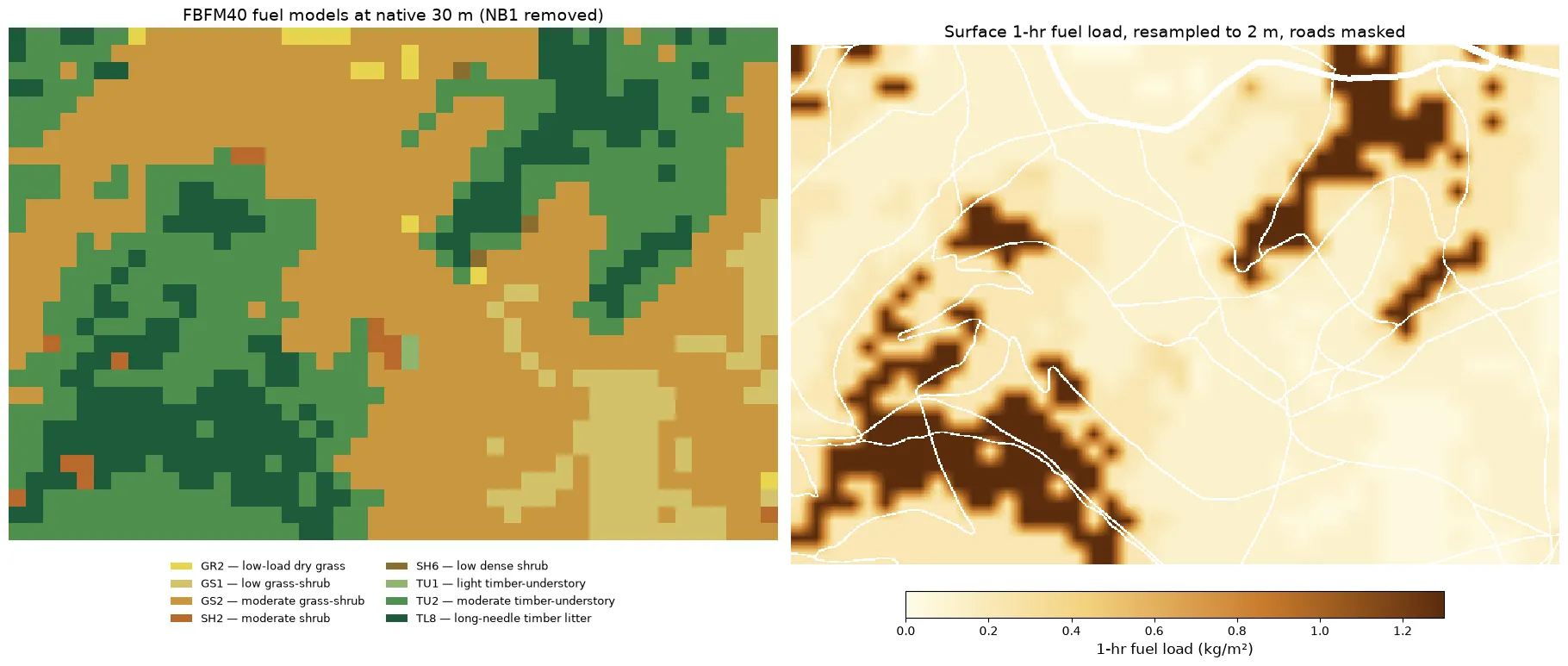
Step 3, before and after. Left, the categorical FBFM40 grid at
LANDFIRE’s native 30 m, with the urban corridor already filled in by
its burnable neighbors. Right, the surface fuel load after lookup and
resampling — the 30 m steps have become smooth gradients on the 2 m
lattice, grassy slopes near 0.2 kg/m², timber litter near 1.3 kg/m² —
and the road mask cuts the white lines through it at the road’s real
width: those cells are exactly 0.
Step 4 — Build the canopy fuel grid
Section titled “Step 4 — Build the canopy fuel grid”The 3-D canopy is four chained builds: a canopy height model (a raster of vegetation height from NAIP aerial imagery), a tree inventory detected from it (one stem per treetop, with roadside trees removed), a GDAM allometry pass that fills in the morphology a height model can’t see, and a voxel grid that turns those stems into per-cell bulk density, moisture, and SAVR.
Build the canopy height model
Section titled “Build the canopy height model”NAIP imagery is processed by a deep-learning model into a ~0.6 m canopy height surface — fine enough that individual crowns stand out as peaks:
curl -X 'POST' \ 'https://api-v2-prod-nyvjyh5ywa-uw.a.run.app/domains/your-domain-id/grids/canopy/naip' \ -H 'accept: application/json' \ -H 'api-key: my-api-key' \ -H 'Content-Type: application/json' \ -d '{ "name": "NAIP CHM"}'chm = ff.grids.create_canopy_height_grid_from_naip_chm(domain, name="NAIP CHM")chm.wait(){ "id": "your-chm-grid-id", "domain_id": "your-domain-id", "name": "NAIP CHM", "description": "", "status": "completed", "progress": { "percent": 100, "message": "Complete" }, "created_on": "2026-08-13T14:57:48.351613Z", "modified_on": "2026-08-13T14:58:22.149166Z", "checksum": "a66d1dc081b54f008cd0ed0589438ee7", "source": { "tile_metadata": { "acquisition_dates": null, "tile_count": 1, "tiles": [ "https://rangeland.ntsg.umt.edu/data/naip-chm/2023/11/m_4611416_nw_11_060_20231019_20240103_chm.tif" ], "tile_source": null, "native_crs": "EPSG:32611" }, "product": "naip", "description": "NAIP high-resolution canopy height model at ~0.6m resolution (CONUS)", "name": "canopy", "alignment": { "resolution": null, "method": null, "target": "domain" }, "extent_buffer_cells": 0 }, "modifications": [], "bands": [ { "key": "chm", "type": "continuous", "unit": "m", "index": 0, "nodata": null } ], "georeference": { "crs": "EPSG:32611", "transform": [ 0.5997260672151095, 0.0, 720226.0, 0.0, -0.5997260672150779, 5190646.595949142 ], "shape": [1475, 2181] }, "error": null, "chunks": { "shape": [512, 512], "count": 15, "count_by_axis": { "y": 3, "x": 5 } }, "tags": []}Record the grid id: your-chm-grid-id.
Detect trees, removing roadside stems
Section titled “Detect trees, removing roadside stems”Run individual-tree detection over the CHM: the local-maxima filter (lmf)
places one tree at each canopy peak taller than 2 m, and the
modifications rule drops every detected tree within 5 m of a road:
curl -X 'POST' \ 'https://api-v2-prod-nyvjyh5ywa-uw.a.run.app/domains/your-domain-id/inventories/tree/chm' \ -H 'accept: application/json' \ -H 'api-key: my-api-key' \ -H 'Content-Type: application/json' \ -d '{ "name": "Tree inventory from CHM (trees near roads removed)", "source_chm_grid_id": "your-chm-grid-id", "algorithm": { "name": "lmf", "min_height": 2, "footprint_size": 3 }, "modifications": [ { "conditions": [ {"source": "feature", "operator": "within", "feature_id": "your-road-feature-id", "buffer_m": 5} ], "actions": [ {"modifier": "remove"} ] } ]}'from fastfuels_sdk.v2.client_library.models import StemIsolationLmf
detected = ff.inventories.create_tree_inventory_from_chm_grid( domain, chm, algorithm=StemIsolationLmf(min_height=2, footprint_size=3), modifications=[ff.remove_trees(ff.tree_within(road, buffer_m=5))], name="Tree inventory from CHM (trees near roads removed)",){ "id": "your-chm-inventory-id", "domain_id": "your-domain-id", "type": "tree", "name": "Tree inventory from CHM (trees near roads removed)", "description": "", "status": "completed", "progress": { "percent": 100, "message": "Complete" }, "created_on": "2026-08-13T14:59:03.709783Z", "modified_on": "2026-08-13T14:59:11.838657Z", "checksum": "229e8297140944ebb085823bb8face01", "source": { "source_chm_grid_id": "your-chm-grid-id", "name": "chm", "source_chm_grid_checksum": "a66d1dc081b54f008cd0ed0589438ee7", "algorithm": { "footprint_size": 3, "name": "lmf", "min_height": 2.0, "max_height": 120.0 } }, "modifications": [ { "conditions": [ { "source": "feature", "operator": "within", "feature_id": "your-road-feature-id", "buffer_m": 5.0 } ], "actions": [ { "modifier": "remove" } ] } ], "treatments": [], "columns": [ { "key": "x", "type": "continuous", "unit": "m" }, { "key": "y", "type": "continuous", "unit": "m" }, { "key": "height", "type": "continuous", "unit": "m" } ], "forestry_metrics": null, "georeference": { "crs": "EPSG:32611", "bounds": [720226.0, 5189762.0, 721534.0, 5190646.0] }, "error": null, "tags": []}Record the inventory id: your-chm-inventory-id, and poll it to
completed:
curl -X 'GET' \ 'https://api-v2-prod-nyvjyh5ywa-uw.a.run.app/domains/your-domain-id/inventories/your-chm-inventory-id' \ -H 'accept: application/json' \ -H 'api-key: my-api-key'detected.wait()On this CHM the filter detects 9,227 treetops; removing those within
5 m of a road leaves 8,023 (1,204 trees dropped). These are overstory
detections — the trees a camera can see from above — and each carries only
x, y, and height, the observables a height model provides.
Fill in morphology with GDAM allometry
Section titled “Fill in morphology with GDAM allometry”Voxelization needs each tree’s dbh, crown_ratio, and species — none of
which a CHM observes. GDAM (a Generalized Dendro Allometric Model)
imputes them from each tree’s position and height, writing a new, completed
inventory:
curl -X 'POST' \ 'https://api-v2-prod-nyvjyh5ywa-uw.a.run.app/domains/your-domain-id/inventories/tree/allometry/gdam' \ -H 'accept: application/json' \ -H 'api-key: my-api-key' \ -H 'Content-Type: application/json' \ -d '{ "name": "Tree inventory completed with GDAM allometry", "source_tree_inventory_id": "your-chm-inventory-id"}'inventory = ff.inventories.create_tree_inventory_from_gdam( domain, detected, name="Tree inventory completed with GDAM allometry",)inventory.wait(){ "id": "your-inventory-id", "domain_id": "your-domain-id", "type": "tree", "name": "Tree inventory completed with GDAM allometry", "description": "", "status": "completed", "progress": { "percent": 100, "message": "Complete" }, "created_on": "2026-08-13T14:59:15.283500Z", "modified_on": "2026-08-13T15:00:10.891663Z", "checksum": null, "source": { "source_tree_inventory_id": "your-chm-inventory-id", "name": "gdam", "source_tree_inventory_checksum": "229e8297140944ebb085823bb8face01", "impute_columns": ["dbh", "crown_ratio", "fia_species_code"] }, "modifications": [], "treatments": [], "columns": [ { "key": "x", "type": "continuous", "unit": "m" }, { "key": "y", "type": "continuous", "unit": "m" }, { "key": "height", "type": "continuous", "unit": "m" }, { "key": "dbh", "type": "continuous", "unit": "cm" }, { "key": "crown_ratio", "type": "continuous", "unit": null }, { "key": "fia_species_code", "type": "categorical", "unit": null } ], "forestry_metrics": { "type": "tree", "tree_count": 8023, "basal_area_per_area": 11.90157691588496, "tree_density": 28.079949137418463, "quadratic_mean_diameter": 8.815367066950966, "dominant_species_groups": [ { "spgrpcd": 2, "name": "Douglas-fir", "basal_area_share": 0.7340371076051233 }, { "spgrpcd": 3, "name": "True fir/hemlock", "basal_area_share": 0.26596289239487675 } ] }, "georeference": { "crs": "EPSG:32611", "bounds": [720226.0, 5189762.0, 721534.0, 5190646.0] }, "error": null, "tags": []}Record the new inventory id — this completed inventory, not the raw
detection, is what gets voxelized: your-inventory-id. Poll it to
completed the same way; all 8,023 trees come back, each now carrying
x, y, height plus the imputed dbh, crown_ratio, and
fia_species_code. See
Complete a tree inventory with GDAM allometry
for what’s imputed and what isn’t.
Voxelize the canopy
Section titled “Voxelize the canopy”Turn the stems into a 3-D grid. resolution is 2 m horizontal and 1 m
vertical (the fire grid’s cell size), and bands are exactly the canopy
quantities the export needs. The biomass_source derives foliage bulk
density from National-Scale Volume and Biomass (nsvb) allometric equations:
curl -X 'POST' \ 'https://api-v2-prod-nyvjyh5ywa-uw.a.run.app/domains/your-domain-id/grids/voxelize/inventory/tree' \ -H 'accept: application/json' \ -H 'api-key: my-api-key' \ -H 'Content-Type: application/json' \ -d '{ "name": "Canopy fuel voxels", "source_inventory_id": "your-inventory-id", "resolution": { "horizontal": 2, "vertical": 1 }, "bands": ["bulk_density.foliage.live", "fuel_moisture.live", "savr.foliage"], "biomass_source": { "type": "allometry", "equations": "nsvb", "components": ["foliage"], "component_states": { "foliage": { "live": 1.0, "dead": 0.0 } } }, "seed": 42}'from fastfuels_sdk.v2.client_library.models import ( AllometryBiomassSource, AllometryBiomassSourceComponentStates, BiomassComponent, BiomassEquations,)
# Voxelization is a method on the completed Inventory, not a grids.create_* call.tree_grid = inventory.voxelize( horizontal_resolution_m=2, vertical_resolution_m=1, bands=["bulk_density.foliage.live", "fuel_moisture.live", "savr.foliage"], biomass_source=AllometryBiomassSource( equations=BiomassEquations.NSVB, components=[BiomassComponent.FOLIAGE], component_states=AllometryBiomassSourceComponentStates.from_dict( {"foliage": {"live": 1.0, "dead": 0.0}}), ), seed=42, name="Canopy fuel voxels",){ "id": "your-tree-grid-id", "domain_id": "your-domain-id", "name": "Canopy fuel voxels", "description": "", "status": "completed", "progress": { "percent": 100, "message": "Complete" }, "created_on": "2026-08-13T15:00:13.966279Z", "modified_on": "2026-08-13T15:00:50.638768Z", "checksum": "5d643f642c04469e8814db3c55d8c391", "source": { "biomass_source": { "type": "allometry", "components": ["foliage"], "component_states": { "foliage": { "dead": 0.0, "live": 1.0 } }, "equations": "nsvb" }, "entity": "tree", "crown_profile_model": "purves", "operation": "voxelize", "resolution": { "vertical": 1.0, "horizontal": 2.0 }, "max_crown_radius_source": { "type": "allometry" }, "moisture_model": { "live": { "value": 100.0, "method": "uniform" } }, "source_inventory_id": "your-inventory-id", "bands": [ "bulk_density.foliage.live", "fuel_moisture.live", "savr.foliage" ], "seed": 42, "input": "inventory" }, "modifications": [], "bands": [ { "key": "bulk_density.foliage.live", "type": "continuous", "unit": "kg/m**3", "index": 0, "nodata": null }, { "key": "fuel_moisture.live", "type": "continuous", "unit": "%", "index": 1, "nodata": null }, { "key": "savr.foliage", "type": "continuous", "unit": "1/m", "index": 2, "nodata": null } ], "georeference": { "crs": "EPSG:32611", "transform": [2.0, 0.0, 720226.0, 0.0, -2.0, 5190646.0], "shape": [33, 442, 654], "z_resolution": 1.0, "z_origin": 0.0 }, "error": null, "chunks": { "shape": [33, 442, 442], "count": 2, "count_by_axis": { "z": 1, "y": 1, "x": 2 } }, "tags": []}Record the canopy grid id: your-tree-grid-id. Its shape is
[33, 442, 654] — 33 vertical layers of 1 m over the 442 × 654 horizontal
grid. That vertical extent becomes the fire grid’s height.
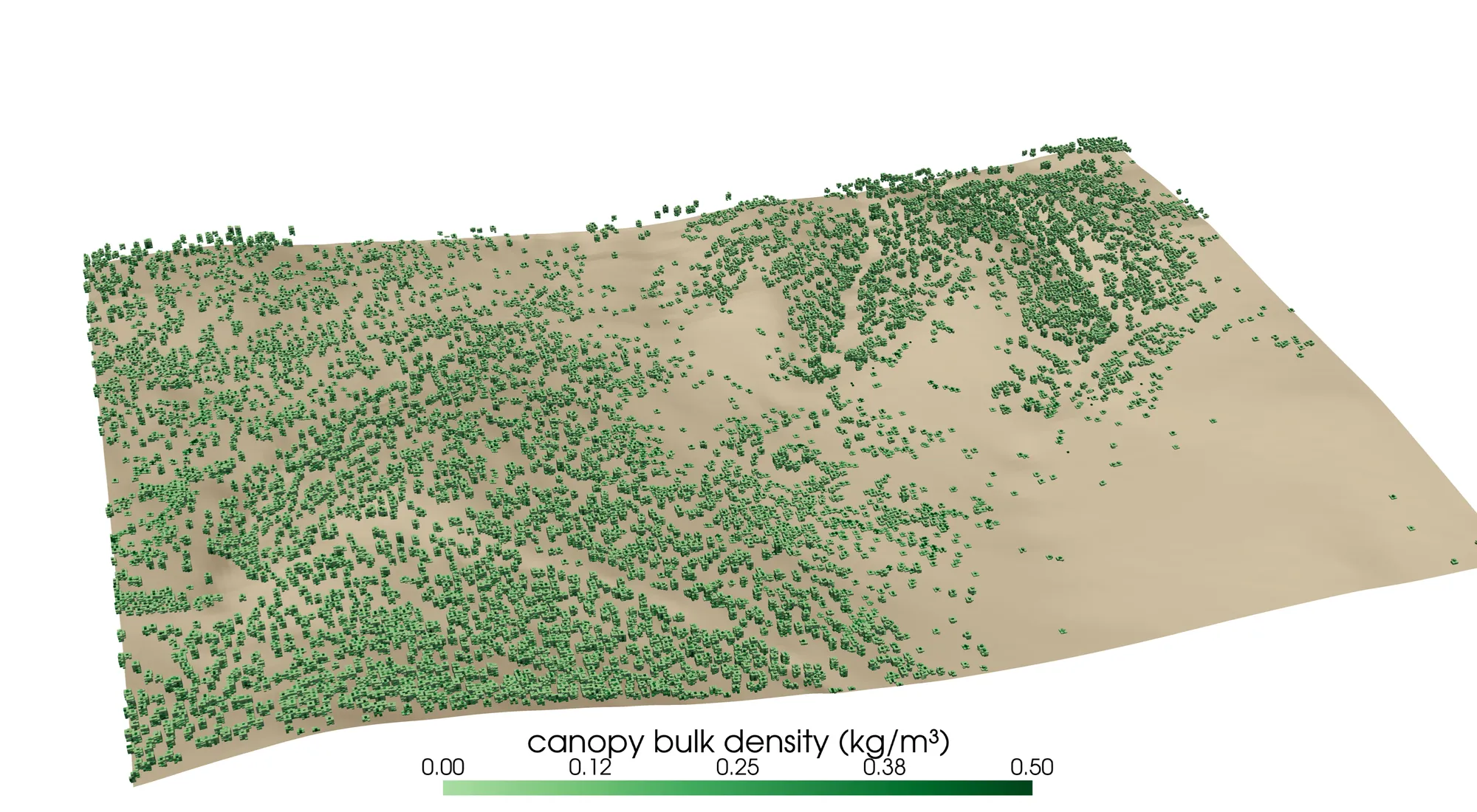
The finished canopy grid, rendered voxel by voxel over the terrain (Step 5’s elevation, used here for display). Each green point is a 2 × 2 × 1 m cell holding foliage — about 208,000 of them, built from the 8,023 detected trees. The timber thickens in the draws and on the north-facing slopes — the TL8/TU2 patches from the surface map — and thins to scattered stems on the open grass slopes toward the east, where the surface grid carries the fuel instead.
Step 5 — Build the topography grid
Section titled “Step 5 — Build the topography grid”QUIC-Fire solves a near-surface wind field over the ground before and during
the burn, and terrain shapes both that wind and the way fire moves across
slopes. The simulation reads that ground as an elevation surface (topo.dat).
Pull elevation from USGS 3DEP, aligned to the same 2 m lattice:
curl -X 'POST' \ 'https://api-v2-prod-nyvjyh5ywa-uw.a.run.app/domains/your-domain-id/grids/topography/3dep' \ -H 'accept: application/json' \ -H 'api-key: my-api-key' \ -H 'Content-Type: application/json' \ -d '{ "name": "Topography (3DEP 10 m)", "source_resolution": 10, "bands": ["elevation"], "alignment": { "target": "domain", "resolution": 2 }}'topography = ff.grids.create_topography_grid_from_3dep( domain, source_resolution_m=10, output_resolution_m=2, bands=["elevation"], name="Topography (3DEP 10 m)",){ "id": "your-topography-grid-id", "domain_id": "your-domain-id", "name": "Topography (3DEP 10 m)", "description": "", "status": "completed", "progress": { "percent": 100, "message": "Complete" }, "created_on": "2026-06-03T17:52:27.489822Z", "modified_on": "2026-06-03T17:52:30.471520Z", "source": { "product": "topography", "tile_metadata": { "native_crs": "EPSG:4326", "tiles": [ "https://prd-tnm.s3.amazonaws.com/StagedProducts/Elevation/13/TIFF/current/n47w115/USGS_13_n47w115.tif" ], "acquisition_dates": null, "tile_source": null, "tile_count": 1 }, "name": "3dep", "description": "3DEP topographic data (elevation, slope, aspect)", "source_resolution": 10, "alignment": { "target": "domain", "resolution": 2.0, "method": null }, "bands": ["elevation"], "extent_buffer_cells": 0 }, "modifications": [], "bands": [ { "key": "elevation", "type": "continuous", "unit": "m", "index": 0, "nodata": -999999.0 } ], "georeference": { "crs": "EPSG:32611", "transform": [2.0, 0.0, 720226.0, 0.0, -2.0, 5190646.0], "shape": [442, 654] }, "error": null, "chunks": { "shape": [512, 512], "count": 2, "count_by_axis": { "x": 2, "y": 1 } }, "tags": []}Record the id: your-topography-grid-id. Across this domain, sampled elevation runs from about 957 m to 1172 m — the ground surface the fire grid sits on.
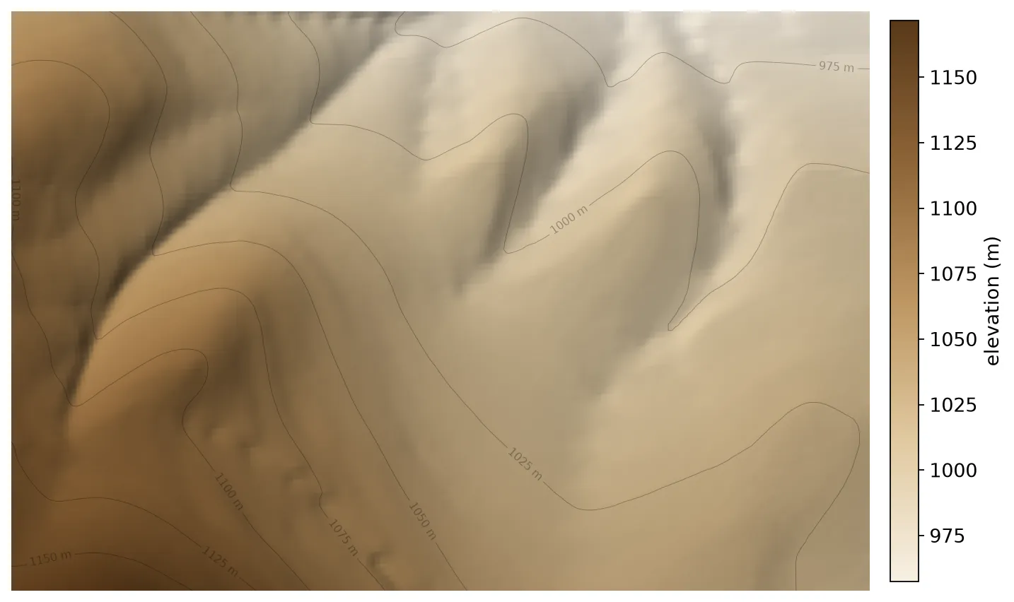
The terrain that shapes the burn: 215 m of relief falling from the southwest corner (1,172 m) to the northeast (957 m), with two steep draws cutting through the middle — the same draws the canopy concentrates in. Fire runs differently up these slopes than across them, which is why QUIC-Fire wants the real surface, not a flat plane.
Step 6 — Build the surface moisture grid
Section titled “Step 6 — Build the surface moisture grid”QUIC-Fire reads a surface fuel-moisture field alongside the loads, as a fraction of dry-fuel mass. The simplest choice is a single uniform value — here, 6%:
curl -X 'POST' \ 'https://api-v2-prod-nyvjyh5ywa-uw.a.run.app/domains/your-domain-id/grids/uniform' \ -H 'accept: application/json' \ -H 'api-key: my-api-key' \ -H 'Content-Type: application/json' \ -d '{ "name": "Surface fuel moisture (uniform 6%)", "resolution": 2, "bands": [ { "key": "fuel_moisture.1hr", "value": 6.0 } ]}'moisture = ff.grids.create_uniform_grid( domain, resolution_m=2, bands={"fuel_moisture.1hr": 6.0}, name="Surface fuel moisture (uniform 6%)",){ "id": "your-moisture-grid-id", "domain_id": "your-domain-id", "name": "Surface fuel moisture (uniform 6%)", "description": "", "status": "completed", "progress": { "percent": 100, "message": "Complete" }, "created_on": "2026-06-03T17:52:28.073960Z", "modified_on": "2026-06-03T17:52:30.691809Z", "source": { "bands": [ { "key": "fuel_moisture.1hr", "value": 6.0 } ], "name": "uniform", "resolution": 2.0 }, "modifications": [], "bands": [ { "key": "fuel_moisture.1hr", "type": "continuous", "unit": "%", "index": 0, "nodata": null } ], "georeference": { "crs": "EPSG:32611", "transform": [2.0, 0.0, 720226.0, 0.0, -2.0, 5190646.0], "shape": [442, 654] }, "error": null, "chunks": { "shape": [512, 512], "count": 2, "count_by_axis": { "x": 2, "y": 1 } }, "tags": []}Record the id: your-moisture-grid-id. That’s the last grid — you now have surface fuel, canopy fuel, terrain, and moisture, all on the same 2 m lattice.
Step 7 — Create the QUIC-Fire export
Section titled “Step 7 — Create the QUIC-Fire export”This is where the pieces come together. The export binds each physical
quantity QUIC-Fire needs to a {grid_id, band} role, and writes the
.dat bundle. Five roles are required (canopy bulk density and moisture;
surface load, depth, and moisture); topography adds topo.dat, and the
SAVR pair adds treesss.dat.
We leave alignment at its default: the domain-anchored fire grid at 2 m
horizontal cells — the resolution QUIC-Fire recommends — and 1 m vertical
layers, which every grid above already matches.
curl -X 'POST' \ 'https://api-v2-prod-nyvjyh5ywa-uw.a.run.app/domains/your-domain-id/grids/exports/quicfire' \ -H 'accept: application/json' \ -H 'api-key: my-api-key' \ -H 'Content-Type: application/json' \ -d '{ "name": "Blue Mountain QUIC-Fire inputs", "canopy_bulk_density": {"grid_id": "your-tree-grid-id", "band": "bulk_density.foliage.live"}, "canopy_moisture": {"grid_id": "your-tree-grid-id", "band": "fuel_moisture.live"}, "canopy_savr": {"grid_id": "your-tree-grid-id", "band": "savr.foliage"}, "surface_fuel_load": {"grid_id": "your-surface-grid-id", "band": "fuel_load.1hr"}, "surface_fuel_depth": {"grid_id": "your-surface-grid-id", "band": "fuel_depth"}, "surface_moisture": {"grid_id": "your-moisture-grid-id", "band": "fuel_moisture.1hr"}, "surface_savr": {"grid_id": "your-surface-grid-id", "band": "savr.1hr"}, "topography": {"grid_id": "your-topography-grid-id", "band": "elevation"}}'# Wait for the four grids still finishing, then bundle. Each quantity is a# (grid, band) pair.for grid in (surface, tree_grid, topography, moisture): grid.wait()
export = ff.exports.create_quicfire_export( domain, canopy_bulk_density=(tree_grid, "bulk_density.foliage.live"), canopy_moisture=(tree_grid, "fuel_moisture.live"), canopy_savr=(tree_grid, "savr.foliage"), surface_fuel_load=(surface, "fuel_load.1hr"), surface_fuel_depth=(surface, "fuel_depth"), surface_moisture=(moisture, "fuel_moisture.1hr"), surface_savr=(surface, "savr.1hr"), topography=(topography, "elevation"), name="Blue Mountain QUIC-Fire inputs",){ "id": "your-export-id", "domain_id": "your-domain-id", "name": "Blue Mountain QUIC-Fire inputs", "description": "", "status": "pending", "progress": null, "created_on": "2026-08-13T15:00:51.323608", "modified_on": "2026-08-13T15:00:51.323608", "source": { "name": "quicfire", "domain_id": "your-domain-id", "alignment": { "target": "domain", "dx": 2.0, "dy": 2.0, "dz": 1.0 }, "canopy_bulk_density": { "grid_id": "your-tree-grid-id", "band": "bulk_density.foliage.live" }, "canopy_moisture": { "grid_id": "your-tree-grid-id", "band": "fuel_moisture.live" }, "canopy_savr": { "grid_id": "your-tree-grid-id", "band": "savr.foliage" }, "surface_fuel_load": { "grid_id": "your-surface-grid-id", "band": "fuel_load.1hr" }, "surface_fuel_depth": { "grid_id": "your-surface-grid-id", "band": "fuel_depth" }, "surface_moisture": { "grid_id": "your-moisture-grid-id", "band": "fuel_moisture.1hr" }, "surface_savr": { "grid_id": "your-surface-grid-id", "band": "savr.1hr" }, "topography": { "grid_id": "your-topography-grid-id", "band": "elevation" }, "rhof_merge": "sum", "moist_merge": "max", "savr_merge": "weighted_avg", "georeference": { "crs": "EPSG:32611", "transform": [2.0, 0.0, 720226.0, 0.0, -2.0, 5190646.0], "shape": [33, 442, 654], "z_resolution": 1.0, "z_origin": 0.0 } }, "signed_url": null, "expires_on": "2026-08-20T15:00:51.323608", "error": null, "tags": []}The 201 echoes a source.georeference — the exact grid the bundle will be
written on, in the same georeference form the grids carry. Its shape is the
familiar [33, 442, 654], the transform holds the 2 m cells, and
z_resolution the 1 m layers. The response also mints an export id.
Record it: your-export-id.
Unlike the grids, the export’s lifecycle lives at /exports/{id} (not under
the domain). Poll it there:
curl -X 'GET' \ 'https://api-v2-prod-nyvjyh5ywa-uw.a.run.app/exports/your-export-id' \ -H 'accept: application/json' \ -H 'api-key: my-api-key'export.wait(){ "id": "your-export-id", "domain_id": "your-domain-id", "name": "Blue Mountain QUIC-Fire inputs", "description": "", "status": "completed", "progress": { "percent": 100, "message": "Complete" }, "created_on": "2026-08-13T15:00:51.323608Z", "modified_on": "2026-08-13T15:01:17.968974Z", "source": { "georeference": { "z_resolution": 1.0, "z_origin": 0.0, "transform": [2.0, 0.0, 720226.0, 0.0, -2.0, 5190646.0], "crs": "EPSG:32611", "shape": [33, 442, 654] }, "surface_fuel_load": { "grid_id": "your-surface-grid-id", "band": "fuel_load.1hr" }, "name": "quicfire", "surface_fuel_depth": { "grid_id": "your-surface-grid-id", "band": "fuel_depth" }, "canopy_savr": { "grid_id": "your-tree-grid-id", "band": "savr.foliage" }, "savr_merge": "weighted_avg", "alignment": { "target": "domain", "dx": 2.0, "dz": 1.0, "dy": 2.0 }, "domain_id": "your-domain-id", "surface_moisture": { "grid_id": "your-moisture-grid-id", "band": "fuel_moisture.1hr" }, "canopy_bulk_density": { "grid_id": "your-tree-grid-id", "band": "bulk_density.foliage.live" }, "canopy_moisture": { "grid_id": "your-tree-grid-id", "band": "fuel_moisture.live" }, "surface_savr": { "grid_id": "your-surface-grid-id", "band": "savr.1hr" }, "rhof_merge": "sum", "topography": { "grid_id": "your-topography-grid-id", "band": "elevation" }, "moist_merge": "max" }, "signed_url": "https://storage.googleapis.com/silvx-fastfuels-exports-v2/your-export-id/Blue_Mountain_QUIC-Fire_inputs.zip?X-Goog-Algorithm=GOOG4-RSA-SHA256&X-Goog-Expires=604800&X-Goog-SignedHeaders=host&X-Goog-Signature=...", "expires_on": "2026-08-20T15:00:51.323608Z", "error": null, "tags": []}When it lands on completed, the response carries a signed_url — a
temporary download link (valid 7 days) for the zipped bundle.
Step 8 — Download and inspect the input files
Section titled “Step 8 — Download and inspect the input files”The completed export carries a signed_url — a temporary link that carries its
own credentials, so no api-key header is needed. In the SDK,
export.to_file(...) follows that link and writes the zip for you; with curl
you download the URL directly:
# When the export status is "completed", copy the `signed_url` from the# response and download it (the URL already carries its own credentials —# no api-key header needed). It expires after 7 days.curl -L 'PASTE_SIGNED_URL_HERE' -o quicfire_inputs.zip
unzip quicfire_inputs.zip -d quicfire_inputsls quicfire_inputs# treesrhof.dat treesmoist.dat treesfueldepth.dat topo.dat# treesss.dat metadata.json domain.geojsonimport zipfile
export.to_file("quicfire_inputs.zip")with zipfile.ZipFile("quicfire_inputs.zip") as archive: archive.extractall("quicfire_inputs") print(archive.namelist())You now have a complete QUIC-Fire input set:
| File | What it holds |
|---|---|
treesrhof.dat | 3-D fuel bulk density (canopy + surface merged at the ground layer) |
treesmoist.dat | 3-D fuel moisture |
treesfueldepth.dat | surface fuel-bed depth (ground layer) |
topo.dat | 2-D terrain elevation |
treesss.dat | 3-D fuel particle size (2 / SAVR) |
metadata.json | the fire-grid dimensions and the export’s provenance |
domain.geojson | the domain footprint, for reference |
The .dat files are Fortran-order binary arrays on the fire grid. Their
dimensions are recorded in metadata.json:
{ "format": "quicfire", "exporter_version": "1", "completed_on": "2026-08-13T15:01:15.153486+00:00", "fire_grid": { "nx": 654, "ny": 442, "nz": 33, "dx": 2.0, "dy": 2.0, "dz": 1.0, "transform": [2.0, 0.0, 720226.0, 0.0, -2.0, 5190646.0], "z_origin": 0.0, "crs": "EPSG:32611" }, "export_id": "your-export-id", "export_name": "Blue Mountain QUIC-Fire inputs", "source": { "topography": { "grid_id": "your-topography-grid-id", "band": "elevation" }, "savr_merge": "weighted_avg", "name": "quicfire", "surface_savr": { "grid_id": "your-surface-grid-id", "band": "savr.1hr" }, "surface_fuel_load": { "grid_id": "your-surface-grid-id", "band": "fuel_load.1hr" }, "canopy_moisture": { "grid_id": "your-tree-grid-id", "band": "fuel_moisture.live" }, "canopy_savr": { "grid_id": "your-tree-grid-id", "band": "savr.foliage" }, "surface_moisture": { "grid_id": "your-moisture-grid-id", "band": "fuel_moisture.1hr" }, "surface_fuel_depth": { "grid_id": "your-surface-grid-id", "band": "fuel_depth" }, "alignment": { "dz": 1.0, "dy": 2.0, "dx": 2.0, "target": "domain" }, "domain_id": "your-domain-id", "canopy_bulk_density": { "grid_id": "your-tree-grid-id", "band": "bulk_density.foliage.live" }, "moist_merge": "max", "georeference": { "transform": [2.0, 0.0, 720226.0, 0.0, -2.0, 5190646.0], "crs": "EPSG:32611", "z_origin": 0.0, "z_resolution": 1.0, "shape": [33, 442, 654] }, "rhof_merge": "sum" }}To run the simulation, place these files in your QUIC-Fire case directory
alongside an input deck — the .inp files that set the winds, ignition,
run length, and outputs, plus a gridlist and rasterorigin.txt describing
the fire grid. The
quicfire-tools Python package
writes all of that for you;
Set up a QUIC-Fire simulation with quicfire-tools
walks the exact deck for this export.
The whole pipeline in one script
Section titled “The whole pipeline in one script”Everything above, start to finish — create the domain, extract roads, build
the surface, canopy, terrain, and moisture grids, export, and download the
.dat bundle. Drop in your API key and run it:
"""Build a complete QUIC-Fire input set with the FastFuels v2 SDK.
Creates a domain, masks roads, builds surface + canopy fuels and terrain,then exports the QUIC-Fire .dat files. `resource.wait()` replaces the manualpoll loop; `export.to_file()` replaces the manual signed-URL download."""import zipfile
import fastfuels_sdk.v2 as fffrom fastfuels_sdk.v2.client_library.models import (    StemIsolationLmf,    AllometryBiomassSource,    AllometryBiomassSourceComponentStates,    BiomassComponent,    BiomassEquations,)
ff.set_api_key("my-api-key")
# 1. Domain — Blue Mountain Recreation Area, padded to a clean 2 m lattice.domain = ff.Domain.from_geojson(    {        "type": "FeatureCollection",        "features": [{            "type": "Feature",            "properties": {},            "geometry": {                "type": "Polygon",                "coordinates": [[                    [-114.09545796676623, 46.8324794598619],                    [-114.11217537297199, 46.8324794598619],                    [-114.11217537297199, 46.82496749915157],                    [-114.09545796676623, 46.82496749915157],                    [-114.09545796676623, 46.8324794598619],                ]],            },        }],    },    name="Blue Mountain Recreation Area",    pad_to_resolution=2,)
# 2. Road feature from OpenStreetMap (reused as a mask below).road = ff.features.create_road_feature_from_osm(domain, name="OSM roads")road.wait()
# 3. Surface fuels: FBFM40 -> per-model load lookup -> resample to 2 m, roads zeroed.fbfm = ff.grids.create_fuel_model_grid_from_landfire_fbfm40(    domain, version="2024", remove_non_burnable=["NB1"],    name="FBFM40 fuel model (LANDFIRE 2024, NB1 removed)",)fbfm.wait()lookup = ff.grids.create_fuel_grid_from_fbfm40_lookup(    fbfm, bands=["fuel_load.1hr", "fuel_depth", "savr.1hr"],    name="Surface fuel loads (FBFM40 lookup)",)lookup.wait()surface = lookup.resample(    output_resolution_m=2,    name="Surface fuels at 2 m, roads masked",    modifications=[        ff.mask(road, ["fuel_load.1hr", "fuel_depth"], 0,                operator="intersects", target="cell"),    ],)
# 4. Canopy fuels: NAIP CHM -> detection (trees near roads removed) -> GDAM -> voxels.chm = ff.grids.create_canopy_height_grid_from_naip_chm(domain, name="NAIP CHM")chm.wait()detection = ff.inventories.create_tree_inventory_from_chm_grid(    domain, chm,    algorithm=StemIsolationLmf(min_height=2, footprint_size=3),    modifications=[ff.remove_trees(ff.tree_within(road, buffer_m=5))],    name="Tree inventory from CHM (trees near roads removed)",)detection.wait()inventory = ff.inventories.create_tree_inventory_from_gdam(    domain, detection, name="Tree inventory completed with GDAM allometry",)inventory.wait()tree_grid = inventory.voxelize(    horizontal_resolution_m=2, vertical_resolution_m=1,    bands=["bulk_density.foliage.live", "fuel_moisture.live", "savr.foliage"],    biomass_source=AllometryBiomassSource(        equations=BiomassEquations.NSVB,        components=[BiomassComponent.FOLIAGE],        component_states=AllometryBiomassSourceComponentStates.from_dict(            {"foliage": {"live": 1.0, "dead": 0.0}}),    ),    seed=42, name="Canopy fuel voxels",)
# 5. Terrain (3DEP elevation) and a uniform surface-moisture grid.topography = ff.grids.create_topography_grid_from_3dep(    domain, source_resolution_m=10, output_resolution_m=2, bands=["elevation"],    name="Topography (3DEP 10 m)",)moisture = ff.grids.create_uniform_grid(    domain, resolution_m=2, bands={"fuel_moisture.1hr": 6.0},    name="Surface fuel moisture (uniform 6%)",)for grid in (surface, tree_grid, topography, moisture):    grid.wait()
# 6. Bundle everything into QUIC-Fire .dat files.export = ff.exports.create_quicfire_export(    domain,    canopy_bulk_density=(tree_grid, "bulk_density.foliage.live"),    canopy_moisture=(tree_grid, "fuel_moisture.live"),    canopy_savr=(tree_grid, "savr.foliage"),    surface_fuel_load=(surface, "fuel_load.1hr"),    surface_fuel_depth=(surface, "fuel_depth"),    surface_moisture=(moisture, "fuel_moisture.1hr"),    surface_savr=(surface, "savr.1hr"),    topography=(topography, "elevation"),    name="Blue Mountain QUIC-Fire inputs",)export.wait()
# 7. Download and unzip the QUIC-Fire input bundle.export.to_file("quicfire_inputs.zip")with zipfile.ZipFile("quicfire_inputs.zip") as archive:    archive.extractall("quicfire_inputs")    print(archive.namelist())# -> ['treesrhof.dat', 'treesmoist.dat', 'treesfueldepth.dat', 'topo.dat',#     'treesss.dat', 'metadata.json', 'domain.geojson']
Next steps
Section titled “Next steps”- Run the simulation yourself. Set up a QUIC-Fire simulation with quicfire-tools builds the tested input deck, runs QUIC-Fire, and reads the outputs back as numpy arrays. The Blue Mountain case study explains the figures produced from one such run and their limitations.
- Tune the fuelscape. Thin fuel along road shoulders instead of zeroing it, or remove only large trees near roads — see Mask a fuel grid with features and Remove trees with features.
- Swap a data source. Build the tree inventory
from TreeMap
or from your own tree list
instead of a CHM. A TreeMap inventory samples stems — understory included —
from the closest-matching FIA field plots, and it arrives with all the
columns voxelization needs (
dbh,crown_ratio, species), so it skips the GDAM step and plugs straight into the voxelizer. An uploaded tree list keeps whatever columns your file had — run GDAM first if it’s only positions and heights, exactly as in Step 4. - Inspect a grid before exporting — fetch and stream the grid data to check values cell by cell.
- Change the horizontal fire grid. Pass an explicit
alignmentto the export for a coarser horizontal simulation (for example,dx: 4anddy: 4); every role grid must still match the resulting lattice. Keepdz: 1when using QUIC-Fire 6.1.1’s FastFuels input convention.