Interpreting a FastFuels export in QUIC-Fire
You are viewing in-progress documentation for v2 (Beta). Switch to the stable version for the current production release.
The QUIC-Fire inputs tutorial builds surface fuel, canopy fuel, terrain, and moisture for the Blue Mountain Recreation Area, then packages them as a FastFuels QUIC-Fire export. We ran that exact export in QUIC-Fire 6.1.1 using the deck from the QUIC-Fire how-to guide: a steady 6 m/s west wind, 6% surface moisture, a north–south line ignition near the upwind edge, and 1,800 seconds of simulated fire time.
At the final output, QUIC-Fire reported that 33.09% of the simulation’s initial modeled fuel mass had burned. That percentage applies only to the fuel represented in the input arrays. It is not a measurement of all vegetation biomass or ecological effects in the real landscape.
Surface-consumption progression
Section titled “Surface-consumption progression”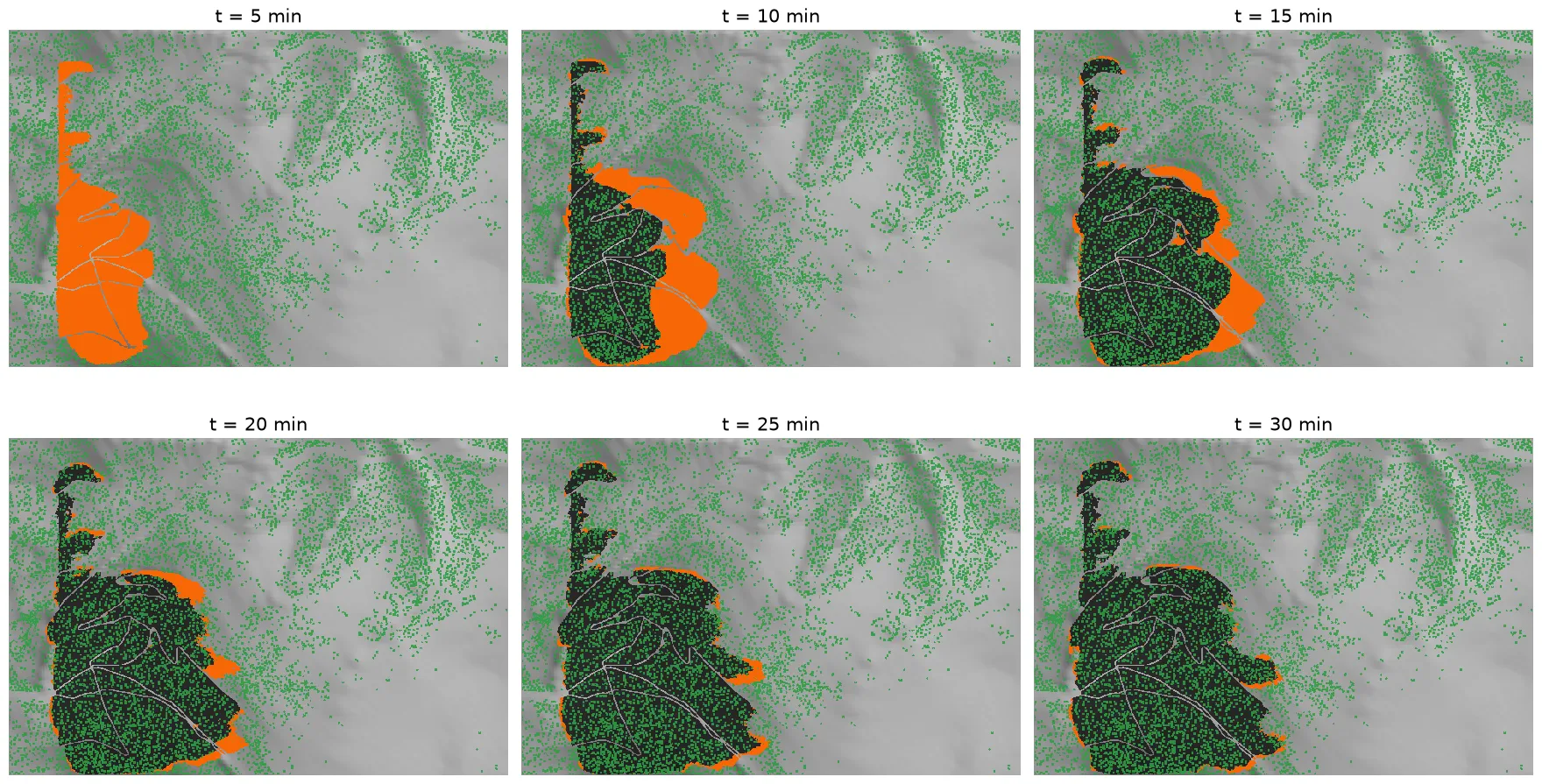
The first half hour of the run, five minutes per frame. Near-black marks surface cells where modeled fuel density has fallen by more than 20%; orange marks cells that first crossed that threshold during the preceding five-minute interval, not the instantaneous fire front. Green marks remaining modeled canopy fuel. The pale road lines are cells assigned zero fuel when the fuelscape was built; this visualization does not test whether a real road would stop fire spread.
The progression is derived from fuels-dens output. Each frame compares the
ground layer with QUIC-Fire’s own output at t = 0, after the model has
initialized the fuels. It does not use reaction rate or fire energy to locate
an active flame front.
Fuel consumed by vertical column
Section titled “Fuel consumed by vertical column”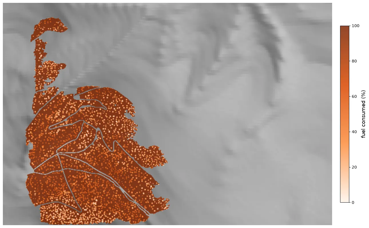
Percent of modeled fuel consumed in each vertical column after 1,800 seconds. The pale speckles coincide with columns where modeled canopy fuel remains at the final output time. Fuel-density output describes modeled fuel consumption; it does not determine tree survival or mortality.
This map normalizes each column independently. A cell with little initial fuel and a cell with substantial initial fuel can therefore display the same percentage. The domain-wide 33.09% result is instead a mass-weighted total reported by QUIC-Fire.
Fire energy in three dimensions
Section titled “Fire energy in three dimensions”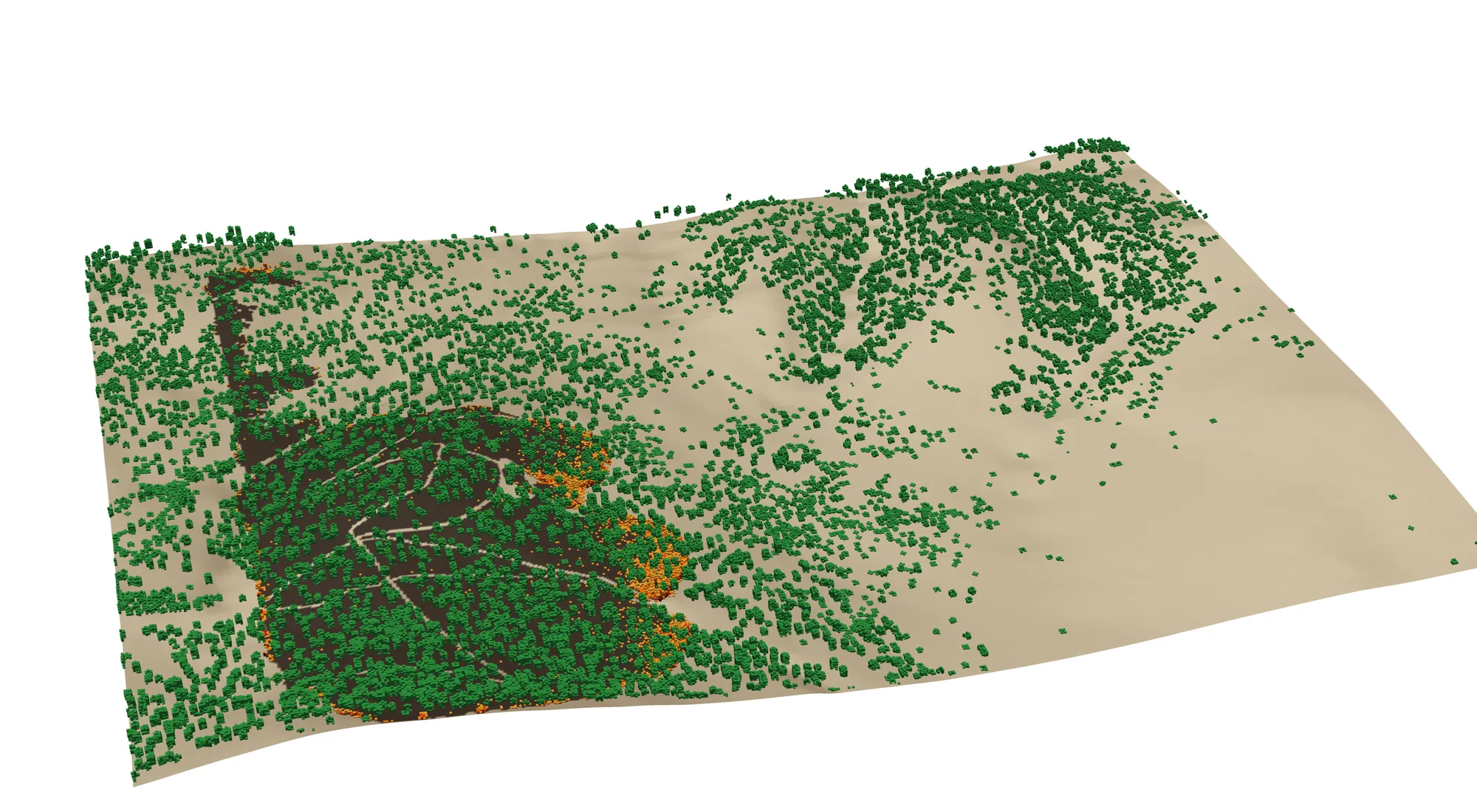
The same simulation in three dimensions at t = 600 seconds. Orange cells are colored by modeled energy released to the atmosphere at that output time; green cells are remaining canopy-fuel voxels. The dark surface uses the same consumption threshold as the progression figure.
The frame combines outputs with the inputs that located them: surface loads, voxelized canopy, and terrain. It shows that the exported arrays can be read and used together by this tested QUIC-Fire configuration. It does not, on its own, establish why the simulated fire followed a particular path or how much any individual input changed the result. Those questions require controlled comparison runs in which one factor changes at a time.
What the case establishes
Section titled “What the case establishes”This case demonstrates that:
- the tutorial’s FastFuels export can be loaded by the tested QUIC-Fire 6.1.1 workflow;
- the surface, canopy, and terrain arrays retain their spatial alignment in the model outputs; and
- QUIC-Fire’s fuel-density, vertically integrated mass-burned, and fire-energy outputs can be read back for analysis.
It does not establish real-world rate of spread, crown or tree survival, the effectiveness of roads as firebreaks, or the separate causal effects of fuel load, moisture, wind, and terrain.
To reproduce the data workflow, start with Create QUIC-Fire simulation inputs. To build and run the tested input deck, follow Set up a QUIC-Fire simulation with quicfire-tools.