From lidar to a tree inventory
You are viewing in-progress documentation for v2 (Beta). Switch to the stable version for the current production release.
Somebody flew an aeroplane over the Blackfoot River valley in Montana in 2021, pointed a laser at the ground, and published the returns. In this tutorial we will turn those returns into a tree inventory: one row per tree, each with a position, a height, a diameter, a crown ratio, and a species.
We will work on about half a square kilometre of river valley, building it in six calls and then inspecting what we made:
| Step | What we do |
|---|---|
| 1 | Create a domain — the patch of ground everything else hangs off |
| 2 | Run a coverage check — is there lidar here, and whose? |
| 3 | Fetch a point cloud — 10.5 million returns, clipped to the domain |
| 4 | Build a canopy height model — the returns rasterized to a 1 m height surface |
| 5 | Detect trees — a detected inventory, one tree per treetop |
| 6 | Fill in the rest — a fully attributed inventory with diameter, crown ratio, and species |
| 7 | Inspect the result, and correct or calibrate it |
Every step after the first is asynchronous: one POST starts it, and you GET
the resource until its status reaches completed. So the rhythm of the whole
tutorial is create → poll → use the id in the next call. In the Python SDK
the poll is resource.wait(), and the Python tabs form one continuous
script — you import and authenticate once in Step 1, then each step keeps the
object it just made and passes it to the next. The whole run takes about three
minutes.
Prerequisites
Section titled “Prerequisites”-
An API key. Create one in the FastFuels web app under your account settings. Set it once here and it propagates to every code block on the page: my-api-key. The SDK reads it via
ff.set_api_key(...)or theFASTFUELS_API_KEYenvironment variable. -
curl, or Python with the FastFuels SDK —pip install fastfuels-sdk(v0.21.0+ for v2).
That’s all — we create everything else as we go.
Step 1 — Create a domain
Section titled “Step 1 — Create a domain”A domain is the georeferenced extent every other resource belongs to. We
POST a GeoJSON FeatureCollection to /domains.
We give the coordinates in UTM zone 12N (EPSG:32612) rather than longitude and
latitude, because we already know exactly which patch of valley we want and the
lidar we are about to fetch is published for it.
curl -X 'POST' \ 'https://api-v2-prod-nyvjyh5ywa-uw.a.run.app/domains' \ -H 'accept: application/json' \ -H 'api-key: my-api-key' \ -H 'Content-Type: application/json' \ -d '{ "type": "FeatureCollection", "name": "Blackfoot River", "description": "About half a square kilometre of the Blackfoot River valley, Montana.", "crs": { "type": "name", "properties": { "name": "EPSG:32612" } }, "features": [ { "type": "Feature", "properties": {}, "geometry": { "type": "Polygon", "coordinates": [[ [294095.0, 5198982.0], [294785.0, 5198982.0], [294785.0, 5199750.0], [294095.0, 5199750.0], [294095.0, 5198982.0] ]] } } ]}'import fastfuels_sdk.v2 as ff
ff.set_api_key("my-api-key")
domain = ff.Domain.from_geojson( { "type": "FeatureCollection", "crs": {"type": "name", "properties": {"name": "EPSG:32612"}}, "features": [ { "type": "Feature", "properties": {}, "geometry": { "type": "Polygon", "coordinates": [ [ [294095.0, 5198982.0], [294785.0, 5198982.0], [294785.0, 5199750.0], [294095.0, 5199750.0], [294095.0, 5198982.0], ] ], }, } ], }, name="Blackfoot River", description="About half a square kilometre of the Blackfoot River valley, Montana.",){ "bbox": [294095.0, 5198982.0, 294785.0, 5199750.0], "type": "FeatureCollection", "features": [ { "type": "Feature", "geometry": { "type": "Polygon", "coordinates": [ [ [294095.0, 5198982.0], [294785.0, 5198982.0], [294785.0, 5199750.0], [294095.0, 5199750.0], [294095.0, 5198982.0] ] ] }, "properties": { "name": "domain" } } ], "name": "Blackfoot River", "description": "About half a square kilometre of the Blackfoot River valley, Montana.", "crs": { "type": "name", "properties": { "name": "EPSG:32612" } }, "tags": [], "id": "your-domain-id", "created_on": "2026-10-13T03:40:42.556785", "modified_on": "2026-10-13T03:40:42.556785"}This one returns immediately — there is no job to wait for. Record the id, since every call below hangs off it: your-domain-id.
Notice the bbox in the response: 294095, 5198982 to 294785, 5199750. That
is 690 m east–west by 768 m north–south, and those numbers reappear in every
resource we build from here.
Step 2 — Ask what lidar is there
Section titled “Step 2 — Ask what lidar is there”Before fetching anything, we ask what the USGS 3D Elevation Program actually holds over this domain. The answer comes back immediately — there is no job to wait for — and asking first is a habit worth keeping: it tells us in advance whether the fetch will succeed, and what it will contain.
curl -X 'GET' \ 'https://api-v2-prod-nyvjyh5ywa-uw.a.run.app/domains/your-domain-id/pointclouds/3dep/coverage' \ -H 'accept: application/json' \ -H 'api-key: my-api-key'coverage = ff.point_clouds.check_3dep_coverage(domain){ "available": true, "coverage_fraction": 1.0, "datasets": [ { "name": "MT_Statewide_P3_4_B21", "url": "https://s3-us-west-2.amazonaws.com/usgs-lidar-public/MT_Statewide_P3_4_B21/ept.json", "contribution_fraction": 1.0, "estimated_density": 14.811981421134373, "estimated_points": 7847291 } ], "estimated_point_count": 7847291}One acquisition, MT_Statewide_P3_4_B21, covers the whole domain on its own —
contribution_fraction is 1.0. That is the simplest case, and it is why this
valley makes a good first lesson.
Note the acquisition’s name. We are going to pin it in the next call.
Step 3 — Fetch the point cloud
Section titled “Step 3 — Fetch the point cloud”Now we pull the returns. Passing datasets pins the fetch to the acquisition we
just found, so this tutorial produces the same cloud today and next year even if
USGS publishes new lidar over the valley.
curl -X 'POST' \ 'https://api-v2-prod-nyvjyh5ywa-uw.a.run.app/domains/your-domain-id/pointclouds/3dep' \ -H 'accept: application/json' \ -H 'api-key: my-api-key' \ -H 'Content-Type: application/json' \ -d '{ "name": "Blackfoot ALS (pinned)", "description": "Pinned to a single 3DEP acquisition so the fetch is reproducible.", "tags": ["blackfoot", "3dep"], "datasets": ["MT_Statewide_P3_4_B21"]}'point_cloud = ff.point_clouds.create_point_cloud_from_3dep( domain, datasets=["MT_Statewide_P3_4_B21"], # optional — pins the acquisition so re-runs are reproducible name="Blackfoot ALS (pinned)", description="Pinned to a single 3DEP acquisition so the fetch is reproducible.", tags=["blackfoot", "3dep"],)Record the id — your-point-cloud-id — and poll until status is
completed. This one takes about twenty seconds.
curl -X 'GET' \ 'https://api-v2-prod-nyvjyh5ywa-uw.a.run.app/domains/your-domain-id/pointclouds/your-point-cloud-id' \ -H 'accept: application/json' \ -H 'api-key: my-api-key'point_cloud.wait(){ "id": "your-point-cloud-id", "domain_id": "your-domain-id", "type": "als", "name": "Blackfoot ALS (pinned)", "description": "Pinned to a single 3DEP acquisition so the fetch is reproducible.", "status": "completed", "progress": { "percent": 100, "message": "Complete" }, "created_on": "2026-10-13T03:29:37.415239Z", "modified_on": "2026-10-13T03:29:47.275218Z", "checksum": "999a8a9fece34397b9db1e5ec47d09c5", "source": { "requested_datasets": ["MT_Statewide_P3_4_B21"], "datasets": ["MT_Statewide_P3_4_B21"], "catalog_fetched_on": "2026-10-13T03:24:38.369894+00:00", "coverage_fraction": 1.0, "name": "3dep" }, "georeference": { "crs": "EPSG:32612", "bounds": [ 294095.0, 5198982.0, 1026.3600000000001, 294785.0, 5199750.0, 1274.19 ] }, "summary": { "point_count": 10512255, "point_classes": [1, 2, 7, 9, 18, 20], "density": 19.837437726449274 }, "error": null, "tags": ["blackfoot", "3dep"]}10,512,255 returns at 19.8 per square metre. Two things in that response are worth stopping on.
First, the coverage check in Step 2 estimated 7,847,291 points and we received 10.5 million — about a third more. The estimate comes from the acquisition’s published average density, and real flight lines overlap, so the estimate is a floor rather than a forecast. See estimate versus delivered for the detail.
Second, point_classes lists 1, 2, 7, 9, 18, 20. Class 2 is ground and class 1
is unclassified — mostly vegetation here. Those two are what the next step needs:
without ground returns, there is no surface to measure height above.
The returns themselves, coloured by height above ground:
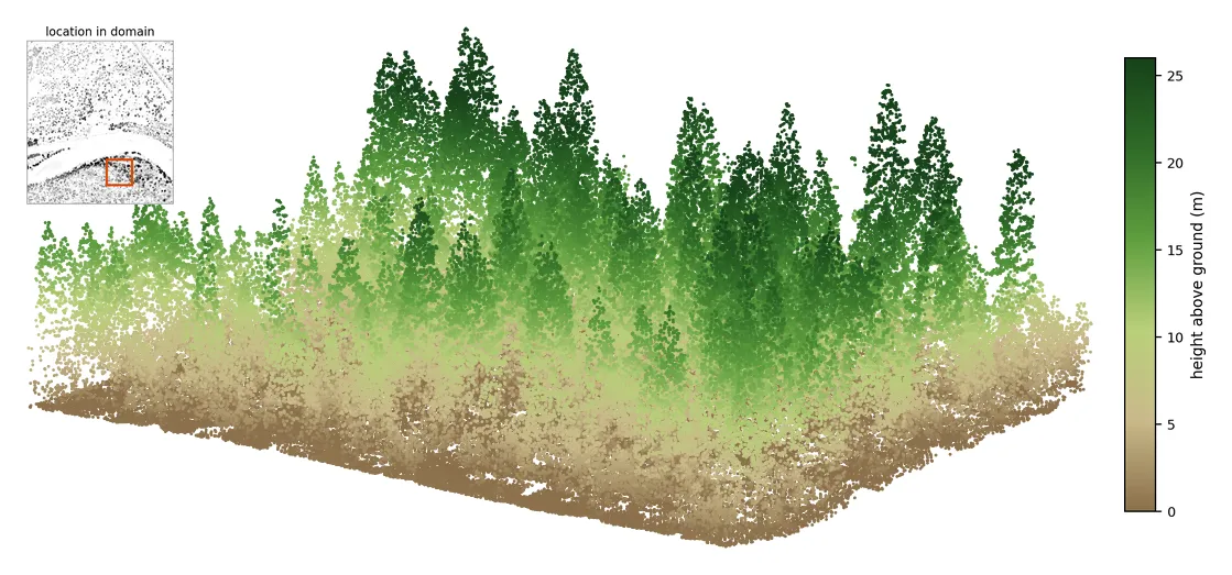
A 120 m block of the domain, holding 358,942 returns — the inset shows where the block sits. Brown points are at ground level, green points are canopy. Thinned for display. The full cloud covers the whole domain and holds 10,512,255 returns.
Step 4 — Build the canopy height model
Section titled “Step 4 — Build the canopy height model”A canopy height model is a raster where each cell holds the height of the tallest return above the ground beneath it. This is the step that turns a cloud of points into a surface we can look for trees in.
curl -X 'POST' \ 'https://api-v2-prod-nyvjyh5ywa-uw.a.run.app/domains/your-domain-id/grids/canopy/point_cloud' \ -H 'accept: application/json' \ -H 'api-key: my-api-key' \ -H 'Content-Type: application/json' \ -d '{ "source_point_cloud_id": "your-point-cloud-id", "name": "Canopy height from 3DEP lidar", "description": "CHM rasterized from the pinned Blackfoot point cloud.", "tags": ["blackfoot", "chm"]}'grid = ff.grids.create_canopy_height_grid_from_point_cloud( point_cloud, name="Canopy height from 3DEP lidar", description="CHM rasterized from the pinned Blackfoot point cloud.", tags=["blackfoot", "chm"],)Record the grid id — your-chm-grid-id — and poll it to completed,
about thirty seconds.
curl -X 'GET' \ 'https://api-v2-prod-nyvjyh5ywa-uw.a.run.app/domains/your-domain-id/grids/your-chm-grid-id' \ -H 'accept: application/json' \ -H 'api-key: my-api-key'grid.wait(){ "id": "your-chm-grid-id", "domain_id": "your-domain-id", "name": "Canopy height from 3DEP lidar", "description": "CHM rasterized from the pinned Blackfoot point cloud.", "status": "completed", "progress": { "percent": 100, "message": "Complete" }, "created_on": "2026-10-13T03:29:48.386716Z", "modified_on": "2026-10-13T03:29:55.888601Z", "checksum": "ad9787cb7abd42ffb6bb598157846b90", "source": { "spike_filter": { "min_prominence_m": 25.0, "min_canopy_footprint_m": 3.0 }, "alignment": { "target": "domain", "resolution": 1.0 }, "aggregation": { "method": "max" }, "name": "canopy", "description": "Canopy height model rasterized from a point cloud", "ground": { "max_ground_distance_m": 35.2, "ground_source": "classification", "ground_coverage": 0.9053 }, "product": "point_cloud", "source_point_cloud_checksum": "999a8a9fece34397b9db1e5ec47d09c5", "extent_buffer_cells": 0, "source_point_cloud_id": "your-point-cloud-id" }, "modifications": [], "bands": [ { "key": "chm", "name": "Canopy Height", "description": "Height above ground of the canopy top.", "type": "continuous", "unit": "m", "index": 0, "nodata": null, "summary": { "type": "continuous", "count": 495428, "nodata_count": 34492, "min": 0.0, "max": 37.64274215698242, "mean": 4.683827075584505, "std": 6.62168395136597 } } ], "georeference": { "crs": "EPSG:32612", "transform": [1.0, 0.0, 294095.0, 0.0, -1.0, 5199750.0], "shape": [768, 690] }, "error": null, "chunks": { "shape": [512, 512], "count": 4, "count_by_axis": { "x": 2, "y": 2 } }, "tags": ["blackfoot", "chm"]}We asked for no resolution, so the grid defaulted to 1 m: a shape of
[768, 690], one cell per metre of the domain.
Stop and read source.ground
Section titled “Stop and read source.ground”This is the most important field on the page, and it is the reason to build a CHM from a cloud rather than upload one you rasterized elsewhere:
"ground": { "max_ground_distance_m": 35.2, "ground_source": "classification", "ground_coverage": 0.9053}A canopy height is a subtraction: the top of the canopy minus the ground under it. If the ground is wrong, every height above it is wrong by the same amount, and nothing downstream can tell. So the grid reports how the ground was established:
ground_source: "classification"— the ground came from returns the vendor labelled as ground (class 2), which is the trustworthy case. Had the cloud carried no usable ground returns, this would readderivedand the ground would be an estimate.ground_coverage: 0.9053— just over 90% of cells had ground returns near enough to use directly. The rest were interpolated.
Look also at the chm band summary: count is 495,428 and nodata_count is
34,492 — about 7% of the domain has no height at all. That is the river. Water
absorbs the pulse and returns nothing, so those cells are genuinely empty rather
than zero. The tallest cell is 37.64 m.
For what each of these fields means in full, and what to do when
ground_coverage is low, see
Read source.ground.
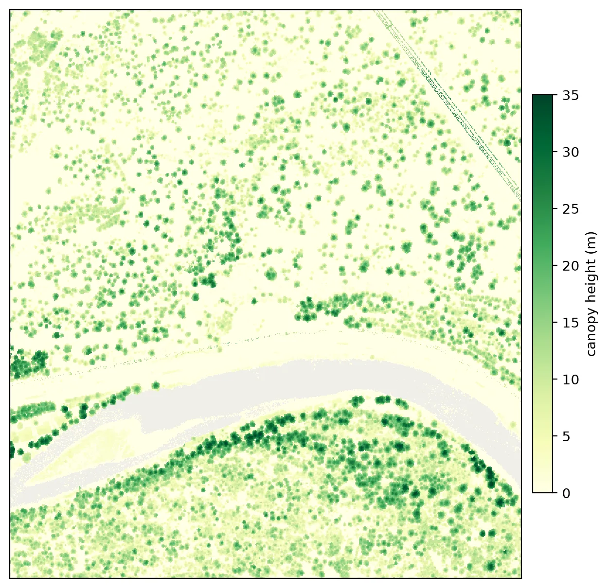
The finished CHM — 10.5 million returns rasterized to 1 m. Every dot is a
crown. The grey ribbon is the Blackfoot River: water absorbs the pulse, so
those cells are the 7% nodata counted above.
Step 5 — Detect the trees
Section titled “Step 5 — Detect the trees”Now we look for treetops. A treetop is a local maximum in the height surface:
a cell taller than everything around it. The lmf algorithm slides a window over
the CHM and places one tree at each peak it finds.
Two parameters shape the result. footprint_size: 5 is the window, in pixels
— on our 1 m grid, a 5 m square. min_height: 2 ignores anything under 2 m, so
we detect trees rather than shrubs.
curl -X 'POST' \ 'https://api-v2-prod-nyvjyh5ywa-uw.a.run.app/domains/your-domain-id/inventories/tree/chm' \ -H 'accept: application/json' \ -H 'api-key: my-api-key' \ -H 'Content-Type: application/json' \ -d '{ "name": "Detected treetops", "source_chm_grid_id": "your-chm-grid-id", "algorithm": { "name": "lmf", "min_height": 2, "footprint_size": 5 }}'from fastfuels_sdk.v2.client_library.models import StemIsolationLmf
detected = ff.inventories.create_tree_inventory_from_chm_grid( domain, grid, algorithm=StemIsolationLmf(min_height=2, footprint_size=5), name="Detected treetops",)Record this inventory’s id — inventory-to-complete — and poll it to
completed, under a minute.
curl -X 'GET' \ 'https://api-v2-prod-nyvjyh5ywa-uw.a.run.app/domains/your-domain-id/inventories/inventory-to-complete' \ -H 'accept: application/json' \ -H 'api-key: my-api-key'detected.wait(){ "id": "inventory-to-complete", "domain_id": "your-domain-id", "type": "tree", "name": "Detected treetops", "description": "", "status": "completed", "progress": { "percent": 100, "message": "Complete" }, "created_on": "2026-10-13T03:29:59.178759Z", "modified_on": "2026-10-13T03:30:00.564929Z", "checksum": "e3f3511f953a4a6aac3580add25ce5e3", "source": { "source_chm_grid_checksum": "ad9787cb7abd42ffb6bb598157846b90", "crown_segmentation": null, "algorithm": { "footprint_size": 5, "min_height": 2.0, "max_height": 120.0, "name": "lmf" }, "source_chm_grid_id": "your-chm-grid-id", "name": "chm" }, "modifications": [], "treatments": [], "columns": [ { "key": "tree_id", "type": "categorical", "unit": null, "summary": { "type": "categorical", "count": 5704, "null_count": 0, "unique_count": 5704 } }, { "key": "x", "type": "continuous", "unit": "m", "summary": { "type": "continuous", "count": 5704, "null_count": 0, "min": 294095.5, "max": 294784.5, "mean": 294432.3616760168, "std": 198.54900263196438 } }, { "key": "y", "type": "continuous", "unit": "m", "summary": { "type": "continuous", "count": 5704, "null_count": 0, "min": 5198982.5, "max": 5199749.5, "mean": 5199325.219845722, "std": 240.39575993484803 } }, { "key": "height", "type": "continuous", "unit": "m", "summary": { "type": "continuous", "count": 5704, "null_count": 0, "min": 2.00134539604187, "max": 37.64274215698242, "mean": 13.151576479011297, "std": 6.974374958995433 } } ], "forestry_metrics": null, "georeference": { "crs": "EPSG:32612", "bounds": [294095.0, 5198982.0, 294785.0, 5199750.0] }, "error": null, "tags": []}5,704 trees. We have gone from a cloud of points to a list of individual stems, and we can already see the shape of the stand: heights run from the 2 m floor we set to 37.64 m, averaging 13.2 m.
Notice that the tallest tree is exactly as tall as the tallest CHM cell — 37.642742 m in both. It has to be: a detected treetop is a cell of the height surface, so detection can never invent a height the CHM did not already hold.
Now notice what is missing. The columns are tree_id, x, y, and height — and
forestry_metrics is null. A height surface seen from above cannot tell us how
thick a trunk is, how far down the crown reaches, or what species we are looking
at, so the API does not guess. Without a diameter there is no basal area, and
without basal area there are no stand metrics.
That is the honest limit of the measurement, and Step 6 is how we get past it.
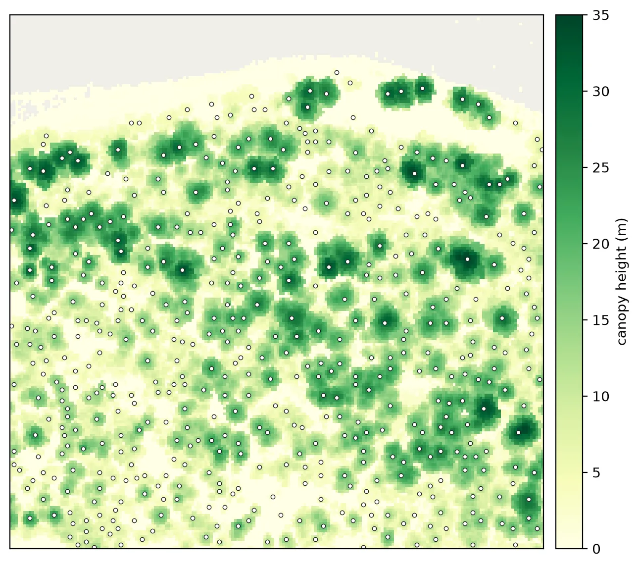
Detected treetops over a 200 m window of dense forest on the south bank — 523 of the 5,704 trees. Each circle is one row of the inventory, placed at a local maximum of the height surface.
Step 6 — Fill in what the CHM could not see
Section titled “Step 6 — Fill in what the CHM could not see”GDAM — a Generalized Dendro Allometric Model — takes each tree’s position and height and imputes the attributes lidar could not observe. We point it at the inventory we just made.
curl -X 'POST' \ 'https://api-v2-prod-nyvjyh5ywa-uw.a.run.app/domains/your-domain-id/inventories/tree/allometry/gdam' \ -H 'accept: application/json' \ -H 'api-key: my-api-key' \ -H 'Content-Type: application/json' \ -d '{ "name": "Fully attributed tree inventory", "source_tree_inventory_id": "inventory-to-complete"}'inventory = ff.inventories.create_tree_inventory_from_gdam( domain, detected, name="Fully attributed tree inventory",)This creates a new inventory rather than modifying the detected one — record
its id as your-inventory-id and poll it to completed, about a minute.
curl -X 'GET' \ 'https://api-v2-prod-nyvjyh5ywa-uw.a.run.app/domains/your-domain-id/inventories/your-inventory-id' \ -H 'accept: application/json' \ -H 'api-key: my-api-key'inventory.wait(){ "id": "your-inventory-id", "domain_id": "your-domain-id", "type": "tree", "name": "Fully attributed tree inventory", "description": "", "status": "completed", "progress": { "percent": 100, "message": "Complete" }, "created_on": "2026-10-13T03:30:04.571781Z", "modified_on": "2026-10-13T03:30:07.078129Z", "checksum": "2bb7b51e9fb742eabf9ca37363333607", "source": { "source_tree_inventory_checksum": "e3f3511f953a4a6aac3580add25ce5e3", "source_tree_inventory_id": "inventory-to-complete", "impute_columns": ["dbh", "crown_ratio", "fia_species_code"], "name": "gdam" }, "modifications": [], "treatments": [], "columns": [ { "key": "tree_id", "type": "categorical", "unit": null, "summary": { "type": "categorical", "count": 5704, "null_count": 0, "unique_count": 5704 } }, { "key": "x", "type": "continuous", "unit": "m", "summary": { "type": "continuous", "count": 5704, "null_count": 0, "min": 294095.5, "max": 294784.5, "mean": 294432.3616760168, "std": 198.5490026319628 } }, { "key": "y", "type": "continuous", "unit": "m", "summary": { "type": "continuous", "count": 5704, "null_count": 0, "min": 5198982.5, "max": 5199749.5, "mean": 5199325.219845722, "std": 240.39575993475967 } }, { "key": "height", "type": "continuous", "unit": "m", "summary": { "type": "continuous", "count": 5704, "null_count": 0, "min": 2.00134539604187, "max": 37.64274215698242, "mean": 13.151576479011297, "std": 6.9743749589954325 } }, { "key": "dbh", "type": "continuous", "unit": "cm", "summary": { "type": "continuous", "count": 5704, "null_count": 0, "min": 11.057536058425903, "max": 52.95517852783203, "mean": 20.168795458054976, "std": 7.704757648933059 } }, { "key": "crown_ratio", "type": "continuous", "unit": null, "summary": { "type": "continuous", "count": 5704, "null_count": 0, "min": 0.4221031188964844, "max": 0.558845329284668, "mean": 0.50615220419655, "std": 0.04045929560294457 } }, { "key": "fia_species_code", "type": "categorical", "unit": null, "summary": { "type": "categorical", "count": 5704, "null_count": 0, "unique_count": 5 } } ], "forestry_metrics": { "type": "tree", "tree_count": 5704, "basal_area_per_area": 17.16558963083773, "tree_density": 43.56008712017423, "quadratic_mean_diameter": 8.500046439321544, "dominant_species_groups": [ { "spgrpcd": 2, "name": "Douglas-fir", "basal_area_share": 0.6599735241735386 }, { "spgrpcd": 3, "name": "True fir/hemlock", "basal_area_share": 0.336330727735944 }, { "spgrpcd": 6, "name": "Aspen/alder/cottonwood-willow", "basal_area_share": 0.003695748090517378 } ] }, "georeference": { "crs": "EPSG:32612", "bounds": [294095.0, 5198982.0, 294785.0, 5199750.0] }, "error": null, "tags": []}Same 5,704 trees, in the same places, at the same heights — with three new
columns: dbh (diameter at breast height, in cm), crown_ratio (the fraction of
the tree’s height that is crown), and fia_species_code.
And forestry_metrics is no longer null. It now carries the numbers a forester
would ask for — note that these follow FIA convention rather than the metric
columns above: basal area in ft²/acre, tree density in trees per acre, and
quadratic mean diameter in inches. Our stand comes out at roughly 44 trees per
acre, a basal area of 17.2 ft²/acre, and a quadratic mean diameter of
8.5 in, with Douglas-fir holding about 66% of the basal area and true
fir/hemlock most of the rest.
Nothing about the stand changed between Step 5 and Step 6. What changed is that the diameters now exist, and every metric that depends on them followed.
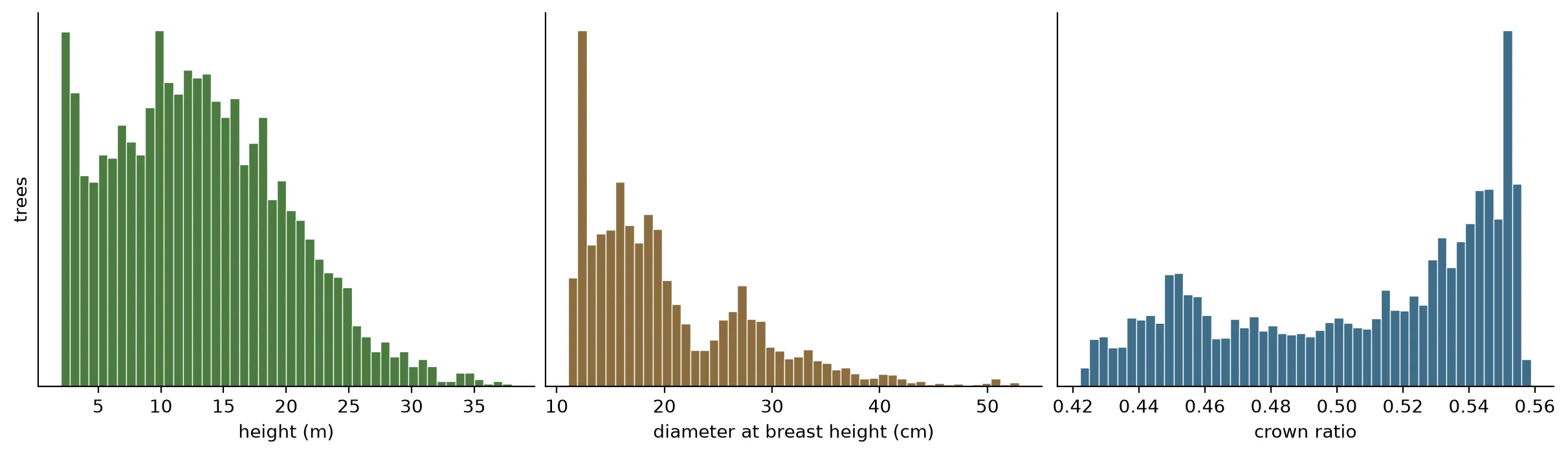
The three columns across all 5,704 trees. Height is measured, and its long tail is the real spread of the stand. Diameter and crown ratio are imputed, and it shows: diameter has a floor near 11 cm, and crown ratio spans barely a tenth. A model asked for a value it cannot observe returns a typical one.
Step 7 — Inspect the trees
Section titled “Step 7 — Inspect the trees”Every column we just added came out of a model, and a model returns a number whether or not that number is right. Before building anything on this inventory, look at it.
The map below draws all 5,704 trees. Click any one to see its stored values, and zoom in where the canopy is dense:
Fetch the same values for the whole inventory with the data endpoints, as Parquet, CSV, or GeoJSON.
What to look for
Section titled “What to look for”- Detections on things that are not trees. Detection runs on a surface model, which records what is physically there rather than what is vegetation. This domain has a clear example — see below.
- Counts that do not match the stand. Our 5,704 detections over 0.53 km² are
44 trees per acre. If your knowledge of the site says otherwise,
footprint_sizeandmin_heightfrom Step 5 are the first things to revisit; Tune CHM detection walks through exporting the CHM and the treetops together and reading the overlay. - Attribute ranges. Across the inventory the imputed columns span
11.1–53.0 cm
dbhand 0.42–0.56crown_ratio. A range far narrower than a real stand’s is expected of an imputed value, but check the centre of it against local data before trusting stand totals. - Species composition. See Species below.
The power line
Section titled “The power line”A transmission line crosses the north-east of this domain, and detection has placed a chain of trees along it:
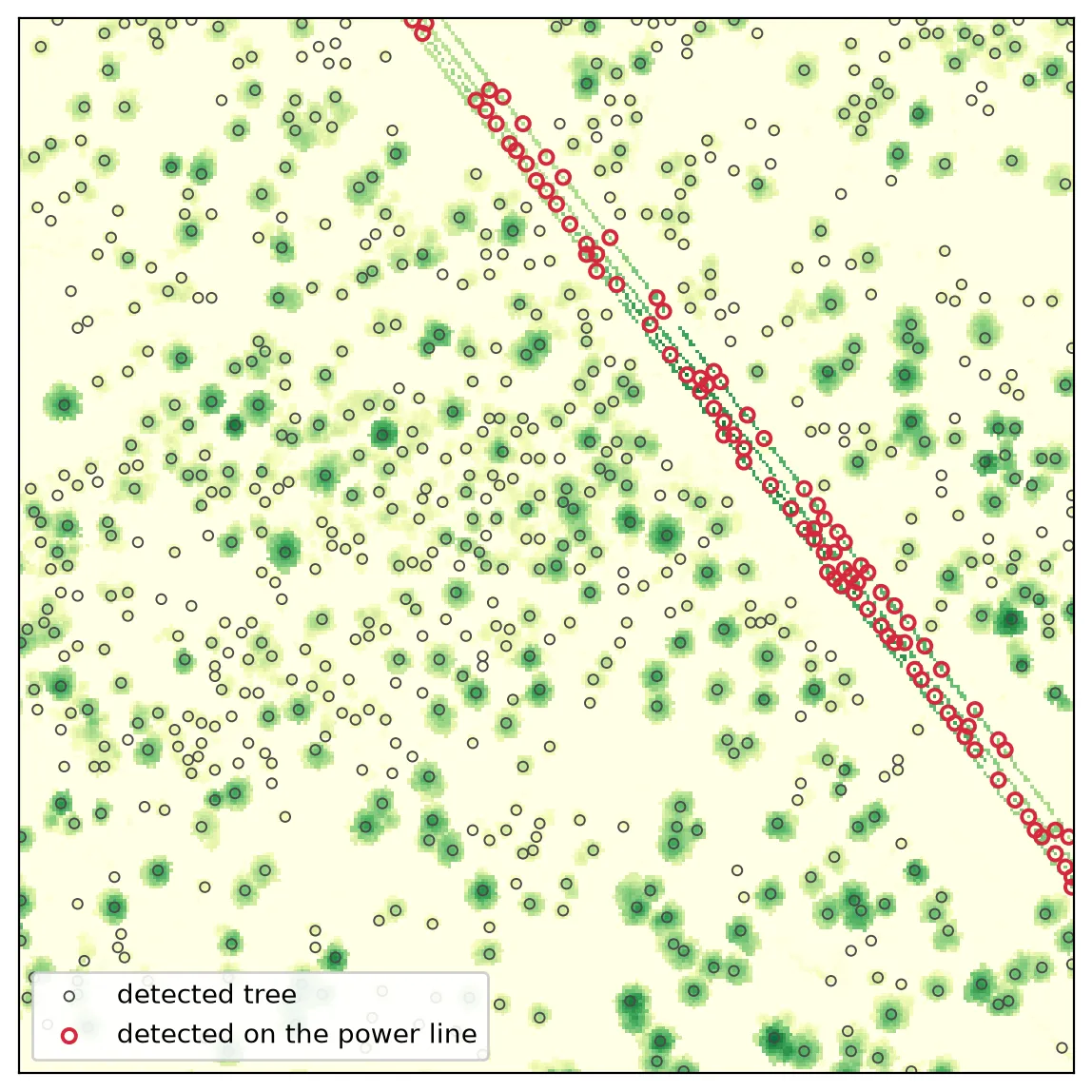
The conductors appear in the CHM as thin parallel lines, and 95 of the 5,704 detections, 1.7% of the inventory, sit on them.
A conductor holds its elevation while the ground falls away beneath it, so it stands well above the ground surface and reads as canopy. In this cloud the vendor left the wires in ASPRS class 1, so they survive into the CHM.
Today this is yours to correct. The detection step has no notion of infrastructure, and nothing in the pipeline will flag it for you — which is the reason to inspect. Remove them with a spatial modification rule: draw a polygon over the corridor and use it as the condition, exactly as Remove trees with road and water features does with a feature. Both the inline-geometry and feature-reference forms are described in About modifications.
Automatic detection of power lines and other structures is something we are looking at for a future release. If it matters for your work, tell us at support.fastfuels@silvxlabs.com — it helps us prioritise.
Species
Section titled “Species”GDAM assigns species from position and height, and this is where its limits are easiest to see. The inventory comes back:
| Species | Trees |
|---|---|
| Douglas-fir | 3,609 |
| western hemlock | 2,069 |
| red alder | 14 |
| Pacific silver fir | 9 |
| mountain hemlock | 3 |
Western hemlock is unlikely on this site, and ponderosa pine — the species most likely to be here — does not appear at all. GDAM is an imputation and it has inaccuracies; treat its species assignment as a starting point to check against what you know of the site, not as an observation.
fia_species_code is a modifiable attribute, so a reassignment is a
modification rule like any other. Conditions on it accept eq and ne only,
since it is categorical. To reassign every western hemlock (FIA code 263) to
ponderosa pine (122):
{ "modifications": [ { "conditions": [ { "attribute": "fia_species_code", "operator": "eq", "value": 263 } ], "actions": [ { "attribute": "fia_species_code", "modifier": "replace", "value": 122 } ] } ]}POST that to .../inventories/{inventory_id}/modifications and poll the
inventory back to completed. See
Modify an inventory
for the full request and the polling loop.
Correcting and calibrating
Section titled “Correcting and calibrating”Nothing here requires rebuilding from the point cloud. Rules are appended to the inventory and applied to its stored trees under the same id, so the order you apply them in is the order they take effect.
| To do this | Use | Where it is documented |
|---|---|---|
| Change the tree count | Re-run detection with different parameters | Tune CHM detection |
| Drop trees by size or attribute | An attribute or expression condition with a remove action | Remove small trees, Remove by expression |
| Drop trees in a place | A spatial condition — inline polygon or a feature | Remove trees under roads or water, Remove trees with features |
| Reassign species | fia_species_code with a replace action | Species above |
| Calibrate a numeric column | multiply, divide, add, subtract, or replace | Scale an attribute |
| Keep the original to compare | Duplicate before modifying | Branch a scenario |
For the concepts behind all of it — conditions, actions, buffer_m, and how
create-time rules differ from in-place ones — read
About modifications.
What we built, and what to question
Section titled “What we built, and what to question”We started from published laser returns and ended with 5,704 trees we can voxelize, treat, or export. It is worth being clear about which parts we measured and which parts we modelled:
| Column | Where it came from |
|---|---|
x, y | Measured — the position of a peak in the height surface |
height | Measured — a return, above a ground surface built from other returns |
dbh, crown_ratio, fia_species_code | Imputed by GDAM from position and height |
Both halves are legitimate; they just carry different kinds of uncertainty, and three things are worth carrying forward:
- A CHM sees the overstory only. Trees beneath the dominant canopy return no visible peak, so 5,704 is a count of what can be seen from above, not of what is standing (why).
- A surface model sees whatever is physically there. The power line in Step 7 is 1.7% of this inventory, on a domain that is otherwise almost all vegetation. A site with buildings would carry more.
- The ground was 90.5% classified, not 100%. The remaining cells rest on an interpolated surface, and their heights inherit that.
The whole pipeline in one script
Section titled “The whole pipeline in one script”Every call above, in order, with the polling folded in:
"""Blackfoot River: 3DEP lidar to a fully attributed tree inventory.
Runs the whole tutorial end to end with the FastFuels v2 SDK. Takes aboutthree minutes. `resource.wait()` replaces the manual poll loop — it blocksuntil the resource reaches `completed`, or raises if it `failed`."""
import fastfuels_sdk.v2 as fffrom fastfuels_sdk.v2.client_library.models import StemIsolationLmf
ff.set_api_key("my-api-key")
# 1 — the domain (Blackfoot River valley, EPSG:32612)domain = ff.Domain.from_geojson(    {        "type": "FeatureCollection",        "crs": {"type": "name", "properties": {"name": "EPSG:32612"}},        "features": [            {                "type": "Feature",                "properties": {},                "geometry": {                    "type": "Polygon",                    "coordinates": [                        [                            [294095.0, 5198982.0],                            [294785.0, 5198982.0],                            [294785.0, 5199750.0],                            [294095.0, 5199750.0],                            [294095.0, 5198982.0],                        ]                    ],                },            }        ],    },    name="Blackfoot River",    description="About half a square kilometre of the Blackfoot River valley, Montana.",)print(f"domain {domain.id}")
# 2 — is there lidar here, and whose?coverage = ff.point_clouds.check_3dep_coverage(domain).to_dict()print(f"coverage {coverage['coverage_fraction']:.0%}, "      f"~{coverage['estimated_point_count']:,} points estimated")
# 3 — fetch it, pinned to one acquisition so the run is reproduciblepoint_cloud = ff.point_clouds.create_point_cloud_from_3dep(    domain,    datasets=["MT_Statewide_P3_4_B21"],    name="Blackfoot ALS (pinned)",    description="Pinned to a single 3DEP acquisition so the fetch is reproducible.",    tags=["blackfoot", "3dep"],)point_cloud.wait()summary = point_cloud.to_dict()["summary"]print(f"point cloud {point_cloud.id}: "      f"{summary['point_count']:,} points, {summary['density']:.1f} pts/m2")
# 4 — rasterize the canopy surfacegrid = ff.grids.create_canopy_height_grid_from_point_cloud(    point_cloud,    name="Canopy height from 3DEP lidar",    description="CHM rasterized from the pinned Blackfoot point cloud.",    tags=["blackfoot", "chm"],)grid.wait()ground = grid.to_dict()["source"]["ground"]print(f"chm {grid.id}: ground from {ground['ground_source']}, "      f"{ground['ground_coverage']:.1%} covered")
# 5 — one tree per treetopdetected = ff.inventories.create_tree_inventory_from_chm_grid(    domain,    grid,    algorithm=StemIsolationLmf(min_height=2, footprint_size=5),    name="Detected treetops",)detected.wait()print(f"detected {detected.id}: "      f"{[c['key'] for c in detected.to_dict()['columns']]}")
# 6 — fill in what the CHM could not seeinventory = ff.inventories.create_tree_inventory_from_gdam(    domain,    detected,    name="Fully attributed tree inventory",)inventory.wait()doc = inventory.to_dict()metrics = doc["forestry_metrics"]print(f"inventory {inventory.id}: {[c['key'] for c in doc['columns']]}")print(f"  {metrics['tree_count']:,} trees, "      f"{metrics['tree_density']:.0f} per acre, "      f"QMD {metrics['quadratic_mean_diameter']:.1f} in")for group in metrics["dominant_species_groups"]:    print(f"  {group['basal_area_share']:.1%} {group['name']}")
Where to go next
Section titled “Where to go next”- Tune the detection — our
footprint_sizeandmin_heightwere reasonable defaults, not tuned ones. Inspect the detection and adjust them until the treetops track the crowns you can see. - Understand what detection can and cannot resolve — how tree detection from a CHM works.
- Build 3D fuel — voxelize the inventory
into a 3D canopy grid, the form a physics-based fire model consumes. The
dbh,crown_ratio, and species columns from Step 6 are exactly what it requires. - Simulate a fire — create QUIC-Fire simulation inputs, which walks the same idea to a full input set.
- Use your own lidar — upload a point cloud instead of fetching one, and rejoin at Step 4.